Download
1 / 32
320 likes | 369 Views
Learn the fundamentals of stereo vision, including epipolar geometry, image rectification, reconstruction, correspondence, and dense and layered stereo. Dive into the Eight-Point Algorithm for computing the Fundamental Matrix and explore techniques for rectifying stereo images for accurate depth perception.

E N D
Stanford CS223B Computer Vision, Winter 2006Lecture 5 Stereo I Stereo Stereo Professor Sebastian Thrun CAs: Dan Maynes-Aminzade, Mitul Saha, Greg Corrado
Vocabulary Quiz • Baseline • Epipole • Fundamental Matrix • Essential Matrix • Stereo Rectification
Stereo Vision: Illustration http://www.well.com/user/jimg/stereo/stereo_list.html
Stereo Example (Stanley Robot) Disparity map
Stereo Vision: Outline • Basic Equations • Epipolar Geometry • Image Rectification • Reconstruction • Correspondence • Dense and Layered Stereo • (Active Range Imaging Techniques)
The Two Problems of Stereo • Correspondence (Wed) • Reconstruction (Today)
Pinhole Camera Model Image plane Focal length f Center of projection
Pinhole Camera Model Image plane
Pinhole Camera Model Image plane
Epipolar Geometry P Pl Pr Yr p p r l Yl Zl Zr Xl fl fr Ol Or Xr
Epipolar Geometry P Pl Pr Epipolar Plane Epipolar Lines p p r l Ol el er Or Epipoles
Epipolar Geometry • Epipolar plane: plane going through point P and the centers of projection (COPs) of the two cameras • Epipoles: The image in one camera of the COP of the other • Epipolar Constraint: Corresponding points must lie on epipolar lines
Essential Matrix Coordinate Transformation: Coplanarity T, Pl, Pl-T: Resolves to Essential Matrix P Pl Pr p p r l Ol el er Or
Essential Matrix Projective Line: Essential Matrix P Pl Pr p p r l Ol el er Or
Fundamental Matrix • Same as Essential Matrix in Camera Pixel Coordinates Pixel coordinates Intrinsic parameters
Computing F: The Eight-Point Algorithm • Problem: Recover F (3-3 matrix of rank 2) • Ides: Get 8 points: • Minimize: • Notice: Argument linear in coefficients of F
Computing F: The Eight-Point Algorithm • Run Singular Value Decomposition of A • Appendix A.6, page 322-325 • See also G. Strang: Linear algebra and its applications Least squares solution: column of V corresponding to the smallest eigenvalue of A
Computing F: The Eight-Point Algorithm • Idea: Compile points into matrix A
Computing F: The Eight-Point Algorithm • Decompose A via SVD: • Solution: F is column of V corresponding to the smallest eigenvector of A • In practice: F will be of rank 3, not 2. Correct by • SVD decomposition of F • Set smallest eigenvalue to 0 • Reconstruct F’
Computing F: The Eight-Point Algorithm • Input: n point correspondences ( n >= 8) • Construct homogeneous system Ax= 0 from • x = (f11,f12, ,f13, f21,f22,f23 f31,f32, f33) : entries in F • Each correspondence give one equation • A is a nx9 matrix • Obtain estimate F^ by SVD of A: • x (up to a scale) is column of V corresponding to the least singular value • Enforce singularity constraint: since Rank (F) = 2 • Compute SVD of F: • Set the smallest singular value to 0: D -> D’ • Correct estimate of F : • Output: the estimate of the fundamental matrix F’ • Similarly we can compute E given intrinsic parameters
Recitification Idea: Align Epipolar Lines with Scan Lines. • Question: What type transformation?
Locating the Epipoles el lies on all the epipolar lines of the left image • Input: Fundamental Matrix F • Find the SVD of F • The epipole el is the column of V corresponding to the null singular value (as shown above) • The epipole er is the column of U corresponding to the null singular value (similar treatment as for el) • Output: Epipole el and er P Pl Pr p p r l Ol el er Or
Stereo Rectification (see Trucco) P Pl Pr Yr p p r l Yl Xl Zl Zr T Ol Or Xr Stereo System with Parallel Optical Axes • Epipoles are at infinity • Horizontal epipolar lines
Reconstruction (3-D): Idealized Pl Pr P p p r l Ol Or
Reconstruction (3-D): Real Pl Pr P p p r l Ol Or See Trucco/Verri, pages 161-171
Summary Stereo Vision (Class 1) • Epipolar Geometry: Corresponding points lie on epipolar line • Essential/Fundamental matrix: Defines this line • Eight-Point Algorithm: Recovers Fundamental matrix • Rectification: Epipolar lines parallel to scanlines • Reconstruction: Minimize quadratic distance