Download
1 / 97
970 likes | 1.13k Views
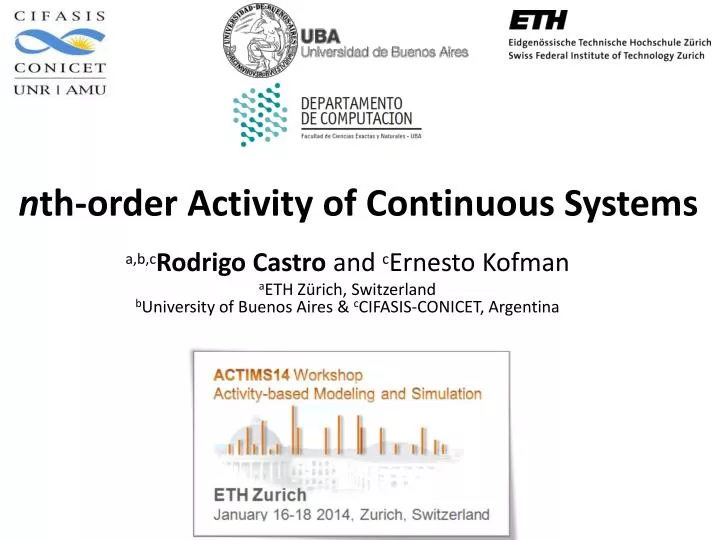
n th-order Activity of Continuous Systems. a,b,c Rodrigo Castro and c Ernesto Kofman a ETH Zürich, Switzerland b University of Buenos Aires & c CIFASIS -CONICET, Argentina. Agenda. Introduction Activity: Original definition Need for an nth-order extension nth-Order Quantization

E N D
nth-order Activity of Continuous Systems • a,b,cRodrigo Castro and cErnestoKofman • aETH Zürich, SwitzerlandbUniversity of Buenos Aires & cCIFASIS-CONICET, Argentina
Agenda • Introduction • Activity: Original definition • Need for an nth-order extension • nth-Order Quantization • Zero (static), First and Second Order • nth-Order Quantization • Quantized State Systems (QSS) • nth-Order Activity • The error perspective • nth-Order error dynamics • Definition of nth-Order Activity • Examples • Example I: 1st. Order Non-stiff system • Example II: 2nd. order Stiff system • Conclusions & Future Work
Activity: Original definition Introduction • The original definition of activity takes into account changes only in the signal values. x1(t) x3(t) x2(t) t0 tf • x1(t0)=x2(t0)=x3(t0) • x1(tf)=x2(tf)=x3(tf)
Activity: Original definition Introduction • The original definition of activity takes into account changes only in the signal values. • As a consequence, for a monotonically increasing or decreasing signal • the activity can be fully determined only by the distance between the final and the initial value, x1(t) x3(t) x2(t) t0 tf • x1(t0)=x2(t0)=x3(t0) • x1(tf)=x2(tf)=x3(tf)
Activity: Original definition Introduction • The original definition of activity takes into account changes only in the signal values. • As a consequence, for a monotonically increasing or decreasing signal • the activity can be fully determined only by the distance between the final and the initial value, • without using at all the information about howit goes from the initial to the final value. x1(t) x3(t) x2(t) t0 tf • x1(t0)=x2(t0)=x3(t0) • x1(tf)=x2(tf)=x3(tf)
Activity: Original definition Introduction • The original definition of activity takes into account changes only in the signal values. • As a consequence, for a monotonically increasing or decreasing signal • the activity can be fully determined only by the distance between the final and the initial value, • without using at all the information about howit goes from the initial to the final value. x1(t) x3(t) x2(t) t0 tf • x1(t0)=x2(t0)=x3(t0) • x1(tf)=x2(tf)=x3(tf) • A1=A2=A3
Activity: Original definition Introduction • The original definition of activity takes into account changes only in the signal values. • As a consequence, for a monotonically increasing or decreasing signal • the activity can be fully determined only by the distance between the final and the initial value, • without using at all the information about howit goes from the initial to the final value. x1(t) x3(t) x2(t) A1=A2=A3 t0 tf • x1(t0)=x2(t0)=x3(t0) • x1(tf)=x2(tf)=x3(tf) • A1=A2=A3
Activity: Original definition Introduction • When a continuous signal is quantized with a zero-order quantization function • we obtain the well-known piecewise constant trajectory xi(t) qi(t) ∆Qi x2(t) m2 ∆Qi m1 m3 t0 tf3 tf2 tf1
Activity: Original definition Introduction • When a continuous signal is quantized with a zero-order quantization function • we obtain the well-known piecewise constant trajectory xi(t) qi(t) ∆Qi x2(t) m2 • For each interval of time at which x(t) is monotonic, the number of signal quantum crossings is: ∆Qi m1 m3 t0 tf3 tf2 tf1
Activity: Original definition Introduction • When a continuous signal is quantized with a zero-order quantization function • we obtain the well-known piecewise constant trajectory xi(t) qi(t) ∆Qi x2(t) m2 • For each interval of time at which x(t) is monotonic, the number of signal quantum crossings is: ∆Qi m1 m3 t0 tf3 tf2 tf1
Activity: Original definition Introduction • When a continuous signal is quantized with a zero-order quantization function • we obtain the well-known piecewise constant trajectory xi(t) qi(t) ∆Qi x2(t) x1(t) m2 • For each interval of time at which x(t) is monotonic, the number of signal quantum crossings is: ∆Qi m1 m3 t0 tf3 tf2 tf1
Activity: Original definition Introduction • When a continuous signal is quantized with a zero-order quantization function • we obtain the well-known piecewise constant trajectory xi(t) qi(t) ∆Qi x3(t) x2(t) x1(t) m2 • For each interval of time at which x(t) is monotonic, the number of signal quantum crossings is: ∆Qi m1 m3 t0 tf3 tf2 tf1
Activity: Original definition Introduction • When a continuous signal is quantized with a zero-order quantization function • we obtain the well-known piecewise constant trajectory xi(t) qi(t) ∆Qi x3(t) x2(t) x1(t) x1(t0)=x2(t0)=x3(t0) x1(tf1)=x2(tf2)=x3(tf3) A1=A2=A3 m2 • For each interval of time at which x(t) is monotonic, the number of signal quantum crossings is: ∆Qi m1 m3 t0 tf3 tf2 tf1
Activity: Original definition Introduction • Zero-order quantization functions are those used in first-order accurate QSS numerical integration methods • QSS1, LIQSS1, CQSS, BQSS xi(t) qi(t) ∆Qi • For each interval of time at which x(t) is monotonic, the number of signal quantum crossings is:
Activity: Original definition Introduction • Zero-order quantization functions are those used in first-order accurate QSS numerical integration methods • QSS1, LIQSS1, CQSS, BQSS • For these methods, the number of signal quantum crossings can establish a lower bound for the number of integration steps • required to approximate the analytical solution • with an accuracy (maximum error) bounded by the quantum size xi(t) qi(t) ∆Qi • For each interval of time at which x(t) is monotonic, the number of signal quantum crossings is:
Need for an nth-order extension Introduction • “Classical”, “Firstorder” Activity • Offers then a link between integration accuracy (Quantum size) and computational effort (# integration steps)
Need for an nth-order extension Introduction • “Classical”, “Firstorder” Activity • Offers then a link between integration accuracy (Quantum size) and computational effort (# integration steps) • Nice features: • Convenient and intuitive visual relation between the solution x(t) and its quantized version q(t) • Can be easily expressed in terms of maxs and mins:
Need for an nth-order extension Introduction • “Classical”, “Firstorder” Activity • Offers then a link between integration accuracy (Quantum size) and computational effort (# integration steps) • Nice features: • Convenient and intuitive visual relation between the solution x(t) and its quantized version q(t) • Can be easily expressed in terms of maxs and mins: • Disadvantages: • It works only for first order accurate methods. • Not valid for higher order accurate methods • Existing QSS methods: QSS 1 to 4, LIQSS 1 to 4, DQSS 1 to 3
Need for an nth-order extension Introduction • “Classical”, “Firstorder” Activity • Offers then a link between integration accuracy (Quantum size) and computational effort (# integration steps) • Nice features: • Convenient and intuitive visual relation between the solution x(t) and its quantized version q(t) • Can be easily expressed in terms of maxs and mins: • Disadvantages: • It works only for first order accurate methods. • Not valid for higher order accurate methods • Existing QSS methods: QSS 1 to 4, LIQSS 1 to 4, DQSS 1 to 3 • Intuition: QSS1 vs. QSS2 • For a given ∆Q, 1st. Order Activity is the same# of Steps is NOT the same QSS1 QSS2 zero order quantization q(t) piecewise constant first order quantization q(t) piecewise linear
Need for an nth-order extension Introduction • “Classical”, “Firstorder” Activity • Offers then a link between integration accuracy (Quantum size) and computational effort (# integration steps) • Nice features: • Convenient and intuitive visual relation between the solution x(t) and its quantized version q(t) • Can be easily expressed in terms of maxs and mins: • Disadvantages: • It works only for first order accurate methods. • Not valid for higher order accurate methods • Existing QSS methods: QSS 1 to 4, LIQSS 1 to 4, DQSS 1 to 3 • Intuition: QSS1 vs. QSS2 • For a given ∆Q, 1st. Order Activity is the same# of Steps is NOT the same • A formal extension forActivity of nth-order is required. QSS1 QSS2 zero order quantization q(t) piecewise constant first order quantization q(t) piecewise linear
Zero (static) and First Order nth-Order Quantization • Quantization: thekey “error-driven” process • Zero-order(static) k1=A1/∆Q
Zero (static) and First Order nth-Order Quantization • Quantization: thekey “error-driven” process • Zero-order(static) polynomial segments j=0,1,2,… k1=A1/∆Q
Zero (static) and First Order nth-Order Quantization • Quantization: thekey “error-driven” process • Zero-order(static) polynomial segments j=0,1,2,… err(t) k1=A1/∆Q
Zero (static) and First Order nth-Order Quantization • Quantization: thekey “error-driven” process • Zero-order(static) polynomial segments j=0,1,2,… q(t)piecewise constant err(t) k1=A1/∆Q
Zero (static) and First Order nth-Order Quantization • Quantization: thekey “error-driven” process • Zero-order(static) • First-order polynomial segments j=0,1,2,… q(t)piecewise constant err(t) k1=A1/∆Q
Zero (static) and First Order nth-Order Quantization • Quantization: thekey “error-driven” process • Zero-order(static) • First-order polynomial segments j=0,1,2,… q(t)piecewise constant err(t) k1=A1/∆Q 1 k2<k1
Zero (static) and First Order nth-Order Quantization • Quantization: thekey “error-driven” process • Zero-order(static) • First-order polynomial segments j=0,1,2,… q(t)piecewise constant err(t) k1=A1/∆Q 1 k2<k1
Zero (static) and First Order nth-Order Quantization • Quantization: thekey “error-driven” process • Zero-order(static) • First-order polynomial segments j=0,1,2,… q(t)piecewise constant err(t) k1=A1/∆Q 1 err(t) k2<k1
Zero (static) and First Order nth-Order Quantization • Quantization: thekey “error-driven” process • Zero-order(static) • First-order polynomial segments j=0,1,2,… q(t)piecewise constant err(t) k1=A1/∆Q 1 q(t)piecewise linear err(t) k2<k1
Zero (static) and First Order nth-Order Quantization • Quantization: thekey “error-driven” process • Zero-order(static) • First-order polynomial segments j=0,1,2,… q(t)piecewise constant err(t) k1=A1/∆Q 1 q(t)piecewise linear err(t) • No visual “quantization grid” available anymore • Now also “how” the signal grows matters (e.g. only one event needed to quantize x(t)=k.t) k2<k1
Second Order nth-Order Quantization • Quantization: thekey “error-driven” process • Second-order k3<k2
Second Order nth-Order Quantization • Quantization: thekey “error-driven” process • Second-order q(t)piecewise parabolic err(t) k3<k2
Second Order nth-Order Quantization • Quantization: thekey “error-driven” process • Second-order • The quantization scheme directly determinesthe number of “polynomial segments” (steps) required q(t)piecewise parabolic err(t) k3<k2
Second Order nth-Order Quantization • Quantization: thekey “error-driven” process • Second-order • The quantization scheme directly determinesthe number of “polynomial segments” (steps) required • We will start with a definition of quantization of order nwhich will lead us to a definition of activity of order n q(t)piecewise parabolic err(t) k3<k2
nth-Order nth-Order Quantization • Quantization: thekey “error-driven” process • nth-order (with n>0)
nth-Order nth-Order Quantization • Quantization: thekey “error-driven” process • nth-order (with n>0) q(t)piecewise nth-order err(t)
nth-Order nth-Order Quantization • Quantization: thekey “error-driven” process • nth-order (with n>0) • m=1,2,…,n q(t)piecewise nth-order err(t)
Quantized State Systems (QSS) nth-Order Quantization • The quantization process keeps track of the dynamics of the error between an input signal and its quantized version • It is the key mechanism used by QSS integrators for error control • QSS: Already discussed in previous presentations. Quick recap:
Quantized State Systems (QSS) nth-Order Quantization • The quantization process keeps track of the dynamics of the error between an input signal and its quantized version • It is the key mechanism used by QSS integrators for error control • QSS: Already discussed in previous presentations. Quick recap: quantized integrator pure integrator
Quantized State Systems (QSS) nth-Order Quantization • The quantization process keeps track of the dynamics of the error between an input signal and its quantized version • It is the key mechanism used by QSS integrators for error control • QSS: Already discussed in previous presentations. Quick recap: quantized integrator pure integrator Event={c0} QSS1
Quantized State Systems (QSS) nth-Order Quantization • The quantization process keeps track of the dynamics of the error between an input signal and its quantized version • It is the key mechanism used by QSS integrators for error control • QSS: Already discussed in previous presentations. Quick recap: quantized integrator pure integrator Event={c0} QSS1 Event={c0,c1} QSS2
Quantized State Systems (QSS) nth-Order Quantization • The quantization process keeps track of the dynamics of the error between an input signal and its quantized version • It is the key mechanism used by QSS integrators for error control • QSS: Already discussed in previous presentations. Quick recap: quantized integrator pure integrator Event={c0} QSS1 Event={c0,c1} QSS2 Event={c0,c1,c2} QSS3
The error perspective nth-Order Activity • The original definition of Activity integrates the rate of changeof the signalx(t):
The error perspective nth-Order Activity • The original definition of Activity integrates the rate of changeof the signalx(t): • When q(t) is the result of a zero-order quantization, the rate of changeof the signal x(t) coincides with the rate of growthof the error |q(t)-x(t)|
The error perspective nth-Order Activity • The original definition of Activity integrates the rate of changeof the signalx(t): • When q(t) is the result of a zero-order quantization, the rate of changeof the signal x(t) coincides with the rate of growthof the error |q(t)-x(t)| • Consequently this formula works:
The error perspective nth-Order Activity • The original definition of Activity integrates the rate of changeof the signalx(t): • When q(t) is the result of a zero-order quantization, the rate of changeof the signal x(t) coincides with the rate of growthof the error |q(t)-x(t)| • Consequently this formula works: • But …
nth-Order error dynamics nth-Order Activity • When q(t) is the result of a high order quantization, the rate of growthof the error |q(t)-x(t)| looks different:
nth-Order error dynamics nth-Order Activity • When q(t) is the result of a high order quantization, the rate of growthof the error |q(t)-x(t)| looks different:
nth-Order error dynamics nth-Order Activity • When q(t) is the result of a high order quantization, the rate of growthof the error |q(t)-x(t)| looks different: =
nth-Order error dynamics nth-Order Activity • When q(t) is the result of a high order quantization, the rate of growthof the error |q(t)-x(t)| looks different: • Let us replace x(t) by its Taylor series expansion: =