Download
1 / 73
730 likes | 858 Views
Chapter 8 – Regression 2. Basic review, estimating the standard error of the estimate and short cut problems and solutions. You can use the regression equation when:. 1. the relationship between X and Y is linear,

E N D
Chapter 8 – Regression 2 Basic review, estimating the standard error of the estimate and short cut problems and solutions.
You can use the regression equation when: 1. the relationship between X and Y is linear, 2. r falls outside the CI.95 around 0.000 and is therefore a statistically significant correlation, and 3. X is within the range of X scores observed in your sample,
tY' = .150 * 0.40 = 0.06 tY' = tY' = .40 * .40 * -1.70 = -0.68 1.70 = 0.68 tY' = r * tX Simple problems using the regression equation
Predictions from Raw Data 1. Calculate the t score for X. 2. Solve the regression equation. 3. Transform the estimated t score for Y into a raw score.
Predicting from and to raw scores Problem: Estimate the midterm point total given a study time of 400 minutes. It is given that the estimated mean of the study time is 560 minutes and the estimated standard deviation is 216.02. (Range = 260-860) It is given that the estimated mean of midterm points is 76 and their estimated standard deviation is 7.98. There were 10 pairs of tX,tY scores The estimated correlation coefficient is .851.
df nonsignificant .05 .01 1 2 3 4 5 6 7 8 9 10 11 12 . . . 100 200 300 500 1000 2000 10000 -.996 to .996 -.949 to .949 -.877 to .877 -.810 to .810 -.753 to .753 -.706 to .706 -.665 to .665 -.631 to .631 -.601 to .601 -.575 to .575 -.552 to .552 -.531 to .531 . . . -.194 to .194 -.137 to .137 -.112 to .112 -.087 to .087 -.061 to .061 -.043 to .043 -.019 to .019 .997 .950 .878 .811 .754 .707 .666 .632 .602 .576 .553 .532 . . . .195 .138 .113 .088 .062 .044 .020 .9999 .990 .959 .917 .874 .834 .798 .765 .735 .708 .684 .661 . . . .254 .181 .148 .115 .081 .058 .026
YES! • r (8) = .851, p < .01 • 400 minutes is inside the range of X scores seen in the random sample (260-860 minutes)
1. Translate raw X to tX score. X X-bar sX (X-X-bar) / sX = tX 400 560 216.02 (400-560)/216.02= -0.74 Predicting from and to raw scores
Use regression equation 2. Find value of tY' r r * tX = tY' .851 .851*-0.74=-0.63
Translate tY' to raw Y' Y sY Y + (tY' * sY) = Y' 76.00 7.98 76.00+(-0.63*7.98) = 70.97
A Caution • Never assume that a correlation will stay linear outside of the range you originally observed. • Therefore, never use the regression equation to make predictions from X values outside of the range you found in your sample. • Example: Basing a prediction of the height of a 50 year old adult based on a study examining the correlation of age and height in a sample composed only of children age 14 or less.
Correlation Characteristics: Which line best shows the relationship between age (X) and height (Y) Linear vs Curvilinear
Reviewing the r table and reporting the results of calculating r from a random sample .
How the r table is laid out: the important columns • Column 1 of the r table shows degrees of freedom for correlation and regression (dfREG) • dfREG=nP-2 • Column 2 shows the CI.95 for varying degrees of freedom • Column 3 shows the absolute value of the r that falls just outside the CI.95. Any r this far or further from 0.000 falsifies the hypothesis that rho=0.000 and can be used in the regression equation to make predictions of Y scores for people who were not in the original sample but who were part of the population from which the sample is drawn.
df nonsignificant .05 .01 1 2 3 4 5 6 7 8 9 10 11 12 . . . 100 200 300 500 1000 2000 10000 -.996 to .996 -.949 to .949 -.877 to .877 -.810 to .810 -.753 to .753 -.706 to .706 -.665 to .665 -.631 to .631 -.601 to .601 -.575 to .575 -.552 to .552 -.531 to .531 . . . -.194 to .194 -.137 to .137 -.112 to .112 -.087 to .087 -.061 to .061 -.043 to .043 -.019 to .019 .997 .950 .878 .811 .754 .707 .666 .632 .602 .576 .553 .532 . . . .195 .138 .113 .088 .062 .044 .020 .9999 .990 .959 .917 .874 .834 .798 .765 .735 .708 .684 .661 . . . .254 .181 .148 .115 .081 .058 .026
If r falls in within the 95% CI around 0.000, then the result is not significant. df nonsignificant .05 .01 1 2 3 4 5 6 7 8 9 10 11 12 . . . 100 200 300 500 1000 2000 10000 -.996 to .996 -.949 to .949 -.877 to .877 -.810 to .810 -.753 to .753 -.706 to .706 -.665 to .665 -.631 to .631 -.601 to .601 -.575 to .575 -.552 to .552 -.531 to .531 . . . -.194 to .194 -.137 to .137 -.112 to .112 -.087 to .087 -.061 to .061 -.043 to .043 -.019 to .019 .997 .950 .878 .811 .754 .707 .666 .632 .602 .576 .553 .532 . . . .195 .138 .113 .088 .062 .044 .020 .9999 .990 .959 .917 .874 .834 .798 .765 .735 .708 .684 .661 . . . .254 .181 .148 .115 .081 .058 .026 Does the absolute value of r equal or exceed the value in this column? Find your degrees of freedom (np-2) in this column You cannot reject the null hypothesis. You can use it in the regression equation to estimate Y scores. r is significant with alpha = .05. You must assume that rho = 0.00. If r is significant you can consider it an unbiased, least squares estimate of rho. alpha = .05.
Can we generalize to the population from the correlation in the sample? • A Type 1 error involves saying that there is a correlation in the population as a whole, when the correlation is actually 0.000 (and the null is true). • We carefully guard against Type 1 error by using significance tests to try to falsify the null hypothesis.
Example : Achovy pizza and horror films, rho=0.000 horror films 7 9 8 6 9 6 5 2 1 6 (scale 0-9) anchovies 7 7 3 3 0 8 4 1 1 1 H1: People who enjoy food with strong flavors also enjoy other strong sensations. H0: There is no relationship between enjoying food with strong flavors and enjoying other strong sensations. Can we reject the null hypothesis?
8 6 4 2 0 0 2 4 6 8 Can we reject the null hypothesis? Pizza Horror films
Can we reject the null hypothesis? We do the math and we find that: r = .352 df = 8
df nonsignificant .05 .01 1 2 3 4 5 6 7 8 9 10 11 12 . . . 100 200 300 500 1000 2000 10000 -.996 to .996 -.949 to .949 -.877 to .877 -.810 to .810 -.753 to .753 -.706 to .706 -.665 to .665 -.631 to .631 -.601 to .601 -.575 to .575 -.552 to .552 -.531 to .531 . . . -.194 to .194 -.137 to .137 -.112 to .112 -.087 to .087 -.061 to .061 -.043 to .043 -.019 to .019 .997 .950 .878 .811 .754 .707 .666 .632 .602 .576 .553 .532 . . . .195 .138 .113 .088 .062 .044 .020 .9999 .990 .959 .917 .874 .834 .798 .765 .735 .708 .684 .661 . . . .254 .181 .148 .115 .081 .058 .026
df nonsignificant .05 .01 1 2 3 4 5 6 7 8 9 10 11 12 . . . 100 200 300 500 1000 2000 10000 -.996 to .996 -.949 to .949 -.877 to .877 -.810 to .810 -.753 to .753 -.706 to .706 -.665 to .665 -.631 to .631 -.601 to .601 -.575 to .575 -.552 to .552 -.531 to .531 . . . -.194 to .194 -.137 to .137 -.112 to .112 -.087 to .087 -.061 to .061 -.043 to .043 -.019 to .019 .997 .950 .878 .811 .754 .707 .666 .632 .602 .576 .553 .532 . . . .195 .138 .113 .088 .062 .044 .020 .9999 .990 .959 .917 .874 .834 .798 .765 .735 .708 .684 .661 . . . .254 .181 .148 .115 .081 .058 .026
df nonsignificant .05 .01 1 2 3 4 5 6 7 8 9 10 11 12 . . . 100 200 300 500 1000 2000 10000 -.996 to .996 -.949 to .949 -.877 to .877 -.810 to .810 -.753 to .753 -.706 to .706 -.665 to .665 -.631 to .631 -.601 to .601 -.575 to .575 -.552 to .552 -.531 to .531 . . . -.194 to .194 -.137 to .137 -.112 to .112 -.087 to .087 -.061 to .061 -.043 to .043 -.019 to .019 .997 .950 .878 .811 .754 .707 .666 .632 .602 .576 .553 .532 . . . .195 .138 .113 .088 .062 .044 .020 .9999 .990 .959 .917 .874 .834 .798 .765 .735 .708 .684 .661 . . . .254 .181 .148 .115 .081 .058 .026
df nonsignificant .05 .01 1 2 3 4 5 6 7 8 9 10 11 12 . . . 100 200 300 500 1000 2000 10000 -.996 to .996 -.949 to .949 -.877 to .877 -.810 to .810 -.753 to .753 -.706 to .706 -.665 to .665 -.631 to .631 -.601 to .601 -.575 to .575 -.552 to .552 -.531 to .531 . . . -.194 to .194 -.137 to .137 -.112 to .112 -.087 to .087 -.061 to .061 -.043 to .043 -.019 to .019 .997 .950 .878 .811 .754 .707 .666 .632 .602 .576 .553 .532 . . . .195 .138 .113 .088 .062 .044 .020 .9999 .990 .959 .917 .874 .834 .798 .765 .735 .708 .684 .661 . . . .254 .181 .148 .115 .081 .058 .026
df nonsignificant .05 .01 1 2 3 4 5 6 7 8 9 10 11 12 . . . 100 200 300 500 1000 2000 10000 -.996 to .996 -.949 to .949 -.877 to .877 -.810 to .810 -.753 to .753 -.706 to .706 -.665 to .665 -.631 to .631 -.601 to .601 -.575 to .575 -.552 to .552 -.531 to .531 . . . -.194 to .194 -.137 to .137 -.112 to .112 -.087 to .087 -.061 to .061 -.043 to .043 -.019 to .019 .997 .950 .878 .811 .754 .707 .666 .632 .602 .576 .553 .532 . . . .195 .138 .113 .088 .062 .044 .020 .9999 .990 .959 .917 .874 .834 .798 .765 .735 .708 .684 .661 . . . .254 .181 .148 .115 .081 .058 .026
This finding falls within the CI.95 around 0.000 • We call such findings “nonsignificant” • Nonsignificant is abbreviated n.s. • We would report these finding as follows • r (8)=0.352, n.s. • Given that it fell inside the CI.95, we must assume that rho actually equals zero and that our sample r is .352 instead of 0.000 solely because of sampling fluctuation. • We go back to predicting that everyone will score at the mean of Y.
In fact, the null hypothesis was correct; rho = 0.000 • I made up that example using numbers randomly selected from a random number table. • So there really was no relationship between the two sets of scores: rho really equaled 0.000 • But samples don’t give you an r of zero, they fluctuate around 0.000 • Significance testing is your protection against mistaking sampling fluctuation for a real correlation. • Significance testing protects against Type 1 error.
We use significance testing to protect us from Type 1 error. • Our sample gave us an r of .352. • Without the r table, we could have thought that far enough from zero to represent a true correlation in the population. • 0.352 was the product only of sampling fluctuation • Significance testing is your protection against mistaking sampling fluctuation for a real correlation. • Significance testing protects against Type 1 error.
How to report a significant r • For example, let’s say that you had a sample (nP=30) and r = -.400 • Looking under nP-2=28 dfREG, we find the interval consistent with the null is between -.360 and +.360 • So we are outside the CI.95 for rho=0.000 • We would write that result as r(28)=-.400, p<.05 • That tells you the dfREG, the value of r, and that you can expect an r that far from 0.000 five or fewer times in 100 when rho = 0.000
Then there is Column 4 • Column 4 shows the values that lie outside a CI.99 • (The CI.99 itself isn’t shown like the CI.95 in Column 2 because it isn’t important enough.) • However, Column 4 gives you bragging rights. • If your r is as far or further from 0.000 as the number in Column 4, you can say there is 1 or fewer chance in 100 of an r being this far from zero (p<.01). • For example, let’s say that you had a sample (nP=30) and r = -.525. • The critical value at .01 is .463. You are further from 0.000 than that.So you can brag. • You write that result as r(28)=-.525, p<.01.
To summarize • If r falls inside the CI.95 around 0.000, it is nonsignificant (n.s.) and you can’t use the regression equation (e.g., r(28)=.300, n.s. • If r falls outside the CI.95, but not as far from 0.000 as the number in Column 4, you have a significant finding and can use the regression equation (e.g., r(28)=-.400,p<.05 • If r is as far or further from zero as the number in Column 4, you can use the regression equation and brag while doing it (e.g., r(28)=-.525, p<.01
df nonsignificant .05 .01 10 11 12 13 14 15 16 17 18 19 . . . 40 50 60 -.575 to .575 -.552 to .552 -.531 to .531 -.513 to .513 -.496 to .496 -.481 to .481 -.467 to .467 -.455 to .455 -.443 to .443 -.432 to .432 . . . -.303 to .303 -.272 to .272 -.249 to .249 .576 .553 .532 .514 .497 .482 .468 .456 .444 .433 . . . .304 .273 .250 .708 .684 .661 .641 .623 .606 .590 .575 .561 .549 . . . .393 .354 .325 Can you reject H0? r = .386 np= 19 dfREG = 17
df nonsignificant .05 .01 10 11 12 13 14 15 16 17 18 19 . . . 40 50 60 -.575 to .575 -.552 to .552 -.531 to .531 -.513 to .513 -.496 to .496 -.481 to .481 -.467 to .467 -.455 to .455 -.443 to .443 -.432 to .432 . . . -.303 to .303 -.272 to .272 -.249 to .249 .576 .553 .532 .514 .497 .482 .468 .456 .444 .433 . . . .304 .273 .250 .708 .684 .661 .641 .623 .606 .590 .575 .561 .549 . . . .393 .354 .325 Can you reject H0? r = -.386 np= 47 dfreg = 45
Improved prediction • If we can use the regression equation rather than the mean to make individualized estimates of Y scores, how much better are our estimates? • We are making predictions about scores on the Y variable from our knowledge of the statistically significant correlation between X & Y and the fact that we know someone’s X score. • The average unsquared error when we predict that everyone will score at the mean of Y equals sY, the ordinary standard deviation of Y. • How much better than that can we do?
Estimating the standard error of the estimate the (very) long way. • Calculate correlation (which includes calculating s for Y). • If the correlation is significant, you can use the regression equation to make individualized predictions of scores on the Y variable. • The average unsquared error of prediction when you do that is called the estimated standard error of the estimate.
Example for Prediction Error • A study was performed to investigate whether the quality of an image affects reading time. • The experimental hypothesis was that reduced quality would slow down reading time. • Quality was measured on a scale of 1 to 10. Reading time was in seconds.
Quality vs Reading Time data: Compute the correlation Quality (scale 1-10) 4.30 4.55 5.55 5.65 6.30 6.45 6.45 Reading time (seconds) 8.1 8.5 7.8 7.3 7.5 7.3 6.0 Is there a relationship? Check for linearity. Compute r.
tX = (X - X) / sX -1.48 -1.19 -0.07 0.05 0.78 0.95 0.95 X - X -1.31 -1.06 -0.06 0.04 0.69 0.84 0.84 (X - X)2 1.71 1.12 0.00 0.00 0.48 0.71 0.71 SSW = 4.73 X=39.25 n= 7 X=5.61 MSW = 4.73/(7-1) = 0.79 s = 0.89 Calculate t scores for X X 4.30 4.55 5.55 5.65 6.30 6.45 6.45
SSW = 3.78 Calculate t scores for Y tY = (Y - Y) / sY 0.76 1.26 0.38 -025 0.00 -0.25 -1.89 Y 8.1 8.5 7.8 7.3 7.5 7.3 6.0 Y - Y 0.60 1.00 0.30 -0.20 0.00 -0.20 -1.50 (Y - Y)2 0.36 1.00 0.09 0.04 0.00 0.04 2.25 Y=52.5 n= 7 Y=7.50 MSW = 3.78/(7-1) = 0.63 sY = 0.794
Plot t scores tX -1.48 -1.19 -0.07 0.05 0.78 0.95 0.95 tY 0.76 1.28 0.39 -0.25 0.00 -0.25 -1.89
(tX - tY)2 = 21.48 Calculate r tX -1.48 -1.19 -0.07 0.05 0.78 0.95 0.95 tY 0.76 1.28 0.39 -0.25 0.00 -0.25 -1.88 tY -tX -2.24 -2.47 -0.46 0.30 0.78 1.20 2.83 (tY -tX)2 5.02 6.10 0.21 0.09 0.61 1.44 8.01 (tX - tY)2 / (nP - 1) = 3.580 = 1 - 1.79 = -0.790 r = 1 - (1/2 * 3.580)
Check whether r is significant r = -0.790 df = nP-2 = 5 Look in r table:With 5 dfREG, the CI.95 goes from -.753 to +.753 is .05 r(5)= -.790, p <.05 r is significant!
We can calculate the Y' for every raw X Y' 8.42 8.23 7.54 7.47 7.01 6.91 6.91 X 4.30 4.55 5.55 5.65 6.30 6.45 6.45
Y 7.5 7.5 7.5 7.5 7.5 7.5 7.5 Can we show mathematically that regression estimates are better than mean estimates? Y' 8.42 8.23 7.54 7.47 7.01 6.91 6.91 Y 8.1 8.5 7.8 7.3 7.5 7.3 6.0 To calculate the standard deviation we take deviations of Y from the mean of Y, square them, add them up, divide by degrees of freedom, and then take the square root. To calculate the standard error of the estimate, sEST, we will take the deviations of each raw Y score from its regression equation estimate, square them, add them up, divide by degrees of freedom, and take the square root. We expect of course that there will be less error if we use regression.
SSRES = 1.49 Estimated standard error of the estimate (Y - Y')2 0.10 0.07 0.07 0.03 0.24 0.15 0.83 Y - Y' -0.32 0.27 0.26 -0.17 0.49 0.39 -0.91 Y' 8.42 8.23 7.54 7.47 7.01 6.91 6.91 Y 8.1 8.5 7.8 7.3 7.5 7.3 6.0 MSRES = 1.49/(7-2) = 0.298 SEST = 0.546
How much better? MSY = 0. 64 MSRES = 0.30 52% less squared error when we use the regression equation instead of the mean to predict Y scores.
How much better is the estimated standard error of the estimate than the estimated standard deviation? SY = 0.80 SEST = 0.546 31% less error of prediction(using unsquared units) when we use the regression equation instead of the mean to predict.