Download
1 / 21
210 likes | 219 Views
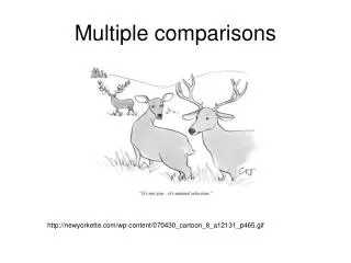
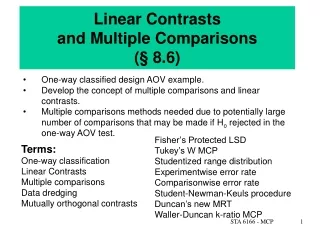
Multiple comparisons. http://newyorkette.com/wp-content/070430_cartoon_8_a12131_p465.gif. How do we decide which means are truly different from one another?. ANOVAs only test the null hypothesis that the treatment means were all sampled from the same distribution…. Two general approaches.

E N D
Multiple comparisons http://newyorkette.com/wp-content/070430_cartoon_8_a12131_p465.gif
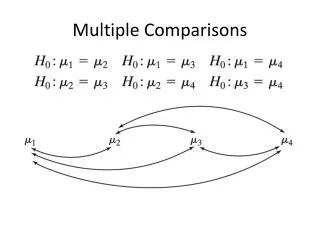
How do we decide which means are truly different from one another? • ANOVAs only test the null hypothesis that the treatment means were all sampled from the same distribution…
Two general approaches • A posteriori comparisons: unplanned, after the fact. • A priori comparisons: planned, before the fact.
Effects of early snowmelt on alpine plant growth Three treatment groups and 4 replicates per treatment: Unmanipulated Heated with permanent solar-powered heating coils that melt spring snow pack earlier in the year than normal Controls, fitted with heating coils that are never activated
ANOVA table for one-way layout P=tail of F-distribution with (a-1) and a(n-1) degrees of freedom
A posteriori comparisons • We will use Tukey’s “honestly significant differences” (HSD) • It controls for the fact that we are carrying out many simultaneous comparisons • the P-value is adjusted downward for each individual test to achieve an experiment-wise error rate of α=0.05
The HSD Where: q= is the value from a statistical table of the studentized range distribution n = sample size
The HSD 2.25, NS 3.25, P<0.05 1, NS So we find significant differences between the control and the heated and no significance between unmanipulated vs. control, or unmanipulated vs. heated…
Dunnett’s test For each treatment vs. control pair, CV= d(m,df) SEt; Where m (number of treatments) includes the control and d is found in tables for Dunnett’s test. Use Dunnett’s test by comparing treatment furthest from control first, then next furthest from control, etc.
Dunnett’s test d-critical(m=3,df=9)=2.61
But… • Occasionally posterior tests may indicate that none of the pairs of means are significantly different from one another, even if the overall F-ratio led to reject the null-hypothesis! • This inconsistence results because the pairwise test are not as powerful as the overall F-ratio itself.
A priori (planned) comparisons • They are more specific • Usually they are more powerful • It forces you to think clearly about which particular treatment differences are of interest
A priori (planned) comparisons • The idea is to establish contrasts, or specified comparisons between particular sets of means that test specific hypothesis • These test must be orthogonal or independent of one another • They should represent a mathematical partitioning of the among group sum of squares
To create a contrast • Assign an number (positive, negative or 0) to each treatment group • The sum of the coefficients for a particular contrast must equal 0 (zero) • Groups of means that are to be averaged together are assigned the same coefficient • Means that are not included in the comparison of a particular contrast are assigned a coefficient of 0
Contrast I (Heated vs. Non-Heated) F-ratio= 20.16/2.17=9.2934 F-critical1,9 =5.12 With 1 df
Contrast I (Heated vs. Non-Heated)using formula for non equal samples F-ratio= 20.16/2.17=9.2934 F-critical1,9 =5.12 With 1 df More information on Sokal and Rohlf (2000) Biometry
Contrast II (Control vs. Unmanipulated) F-ratio= 2/2.17=0.9217 F-critical1,9 =5.12 With 1 df
In order to create additional orthogonal contrasts • If there are a treatment groups, at most there can be (a-1) orthogonal contrasts created (although there are many possible sets of such orthogonal contrasts). • All of the pair-wise cross products must sum to zero. In other words, a pair of contrast Q and R is independent if the sum of the products of their coefficients CQi and CRi equals zero.