Download
1 / 29
310 likes | 446 Views
Rule-Based Classification. Rule-based classifiers, where the learned model is represented as a set of IF-THEN rules. Using IF-THEN Rules for Classification An IF-THEN rule is an expression of the form IF condition THEN conclusion.

E N D
Rule-Based Classification Rule-based classifiers, where the learned model is represented as a set of IF-THEN rules. Using IF-THEN Rules for Classification An IF-THEN rule is an expression of the form IF condition THEN conclusion. R1: IF age = youth AND student = yes THEN buys computer = yes. The “IF”-part of a rule is known as the rule antecedent or precondition. The “THEN”-part is the rule consequent. In the rule antecedent, the condition consists of one or more attribute tests (such as age = youth, and student = yes) that are logically ANDed.
Rule-Based Classification The rule’s consequent contains a class prediction. R1 can also be written as: If the condition in a rule antecedent holds true for a given tuple, we say that the rule antecedent is satisfied and that the rule covers the tuple. A rule R can be assessed by its coverage and accuracy Given a tuple, X, from a class labelled data set, D. let ncoversbe the number of tuples covered by R, ncorrectbe the number of tuples correctly classified by R and |D| be the number of tuples in D. We can define the coverage and accuracy of R as
Rule-Based Classification Consider rule R1, which covers 2 of the 14 tuples. It can correctly classify both tuples. coverage(R1) = 2/14 14.28% accuracy (R1) = 2/2 = 100%.
Rule-Based Classification Let’s see how we can use rule-based classification to predict the class label of a given tuple, X. If a rule is satisfied by X, the rule is said to be triggered. For example, suppose we have We would like to classify X according to buys computer. X satisfies R1, which triggers the rule. If R1 is the only rule satisfied, then the rule fires by returning the class prediction for X.
Rule-Based Classification Triggering does not always mean firing since there may be more than one rule that is satisfied! If more than one rule is triggered, then What if they each specify a different class? We need a conflict resolution strategy to figure out which rule gets to fire and assign its class prediction to X. The size ordering scheme assigns the highest priority to the triggering rule that has the “toughest” requirements. Toughness is measured by the rule antecedent size. That is, the triggering rule with the most attribute tests is fired.
Rule-Based Classification The rule ordering scheme prioritizes the rules beforehand. The ordering may be class based or rule-based. With class-based ordering, the classes are sorted in order of decreasing “importance,” such as by decreasing order of prevalence. That is, all of the rules for the most prevalent (or most frequent) class come first, the rules for the next prevalent class come next, and so on. Within each class, the rules are not ordered—they don’t have to be because they all predict the same class (and so there can be no class conflict!).
Rule-Based Classification With rule-based ordering, the rules are organized into one long priority list, according to some measure of rule quality such as accuracy, coverage, or size or based on advice from domain experts. When rule ordering is used, the rule set is known as a decision list. With rule ordering, the triggering rule that appears earliest in the list has highest priority, and so it gets to fire its class prediction. Any other rule that satisfies X is ignored. Most rule-based classification systems use a class-based rule-ordering strategy.
Rule-Based Classification What if there is no rule satisfied by X? How, then, can we determine the class label of X? In this case, a fallback or default rule can be set up to specify a default class, based on a training set. This may be the class in majority or the majority class of the tuples that were not covered by any rule. The default rule is evaluated at the end, if and only if no other rule covers X. The condition in the default rule is empty. In this way, the rule fires when no other rule is satisfied
Rule-Based Classification Rule Extraction from a Decision Tree Decision trees can become large and difficult to interpret. In comparison with a decision tree, the IF-THEN rules may be easier for humans to understand, particularly if the decision tree is very large. To extract rules from a decision tree, one rule is created for each path from the root to a leaf node. Each splitting criterion along a given path is logically ANDed to form the rule antecedent (“IF” part). The leaf node holds the class prediction, forming the rule consequent (“THEN” part).
Rule-Based Classification Rule Extraction from a Decision Tree
Rule-Based Classification Rule Extraction from a Decision Tree A disjunction (logical OR) is implied between each of the extracted rules. Because the rules are extracted directly from the tree, they are mutually exclusive and exhaustive. By mutually exclusive means that we cannot have rule conflicts here because no two rules will be triggered for the same tuple. By exhaustive, there is one rule for each possible attribute-value combination, so that this set of rules does not require a default rule. Therefore, the order of the rules does not matter—they are unordered.
Rule-Based Classification Rule Extraction from a Decision Tree The rules extracted from decision trees that suffer from subtree repetition and replication can be large and difficult to follow. Although it is easy to extract rules from a decision tree, we may need to do some more work by pruning the resulting rule set. “How can we prune the rule set?” For a given rule antecedent, any condition that does not improve the estimated accuracy of the rule can be pruned, thereby generalizing the rule. C4.5 extracts rules from an unpruned tree, and then prunes the rules using a pessimistic approach similar to its tree pruning method.
Rule-Based Classification Rule Extraction from a Decision Tree Other problems arise during rule pruning, however, as the rules will no longer be mutually exclusive and exhaustive. For conflict resolution, C4.5 adopts a class-based ordering scheme. It groups all rules for a single class together, and then determines a ranking of these class rule sets. Within a rule set, the rules are not ordered. C4.5 orders the class rule sets so as to minimize the number of false-positive errors. The class rule set with the least number of false positives is examined first.
Rule-Based Classification Rule Induction Using a Sequential Covering Algorithm IF-THEN rules can be extracted directly from the training data using a sequential covering algorithm. The general strategy is as follows: Rules are learned one at a time. Each time a rule is learned, the tuples covered by the rule are removed, and the process repeats on the remaining tuples. This sequential learning of rules is in contrast to decision tree induction. Because the path to each leaf in a decision tree corresponds to a rule, we can consider decision tree induction as learning a set of rules simultaneously.
Rule-Based Classification Rule Induction Using a Sequential Covering Algorithm Rules are learned for one class at a time. Ideally, when learning a rule for a class, Ci, we would like the rule to cover all (or many) of the training tuples of class Ci and none (or few) of the tuples from other classes. In this way, the rules learned should be of high accuracy. The rules need not necessarily be of high coverage. The process continues until the terminating condition is met, such as when there are no more training tuples or the quality of a rule returned is below a user-specified threshold.
Rule-Based Classification Rule Induction Using a Sequential Covering Algorithm The Learn_One_Rule procedure finds the “best” rule for the current class, given the current set of training tuples. How are rules learned?” Typically, rules are grown in a general-to-specific manner. We start off with an empty rule and then gradually keep appending attribute tests to it. We append by adding the attribute test as a logical conjunct to the existing condition of the rule antecedent.
Rule Induction Using a Sequential Covering Algorithm Suppose our training set, D, consists of loan application data. Attributes regarding each applicant include their age, income, education level, residence, credit rating, and the term of the loan. The classifying attribute is loan decision, which indicates whether a loan is accepted (considered safe) or rejected (considered risky). To learn a rule for the class “accept,” we start off with the most general rule possible, that is, the condition of the rule antecedent is empty. The rule is: We then consider each possible attribute test that may be added to the rule.
Rule Induction Using a Sequential Covering Algorithm Learn_One_Rule adopts a greedy depth-first strategy. Each time it is faced with adding a new attribute test (conjunct) to the current rule, it picks the one that most improves the rule quality, based on the training samples. suppose Learn One Rule finds that the attribute test income = high best improves the accuracy of our current (empty) rule. We append it to the condition, so that the current rule becomes: IF income = high THEN loan_decision =accept
Rule Induction Using a Sequential Covering Algorithm Each time we add an attribute test to a rule, the resulting rule should cover more of the “accept” tuples. During the next iteration, we again consider the possible attribute tests and end up selecting credit rating = excellent. Our current rule grows to become: The process repeats, where at each step, we continue to greedily grow rules until the resulting rule meets an acceptable quality level.
Prediction “What if we would like to predict a continuous value, rather than a categorical label?” Numeric prediction is the task of predicting continuous (or ordered) values for given input. For example, we may wish to predict the salary of college graduates with 10 years of work experience. By far, the most widely used approach for numeric prediction is regression. It is a statistical methodology that was developed by Sir Frances Galton (1822 – 1911), a mathematician who was also a cousin of Charles Darwin.
Prediction Regression analysis can be used to model the relationship between one or more independentorpredictorvariables and a dependent or responsevariable. In the context of data mining, the predictor variables are the attributes of interest describing the tuple. In general, the values of the predictor variables are known. The response variable is what we want to predict. Given a tuple described by predictor variables, we want to predict the associated value of the response variable.
Linear Regression Straight-line regression analysis involves a response variable, y, and a single predictor variable, x. It is the simplest form of regression, and models y as a linear function of x. That is, y = b + wx where the variance of y is assumed to be constant, and b and w are regression coefficients specifying the Y-intercept and slope of the line, respectively. The regression coefficients, w and b, can also be thought of as weights, so that we can equivalently write y = w0 + w1x
Linear Regression These coefficients can be solved by the method of least squares. Let D be a training set consisting of values of predictor variable, x, for some population and their associated values for response variable, y. The training set contains |D| data points of the form (x1, y1), (x2, y2), . . . ,(x|D| , y|D|) The regression coefficients can be estimated using this method with the following equations:
Multiple Linear Regression Multiple linear regression is an extension of straight-line regression so as to involve more than one predictor variable. It allows response variable y to be modelled as a linear function of, say, n predictor variables or attributes, A1, A2, . . . , An, describing a tuple, X. (That is, X = (x1, x2, : : : , xn).) Our training data set, D, contains data of the form (x1, y1), (x2, y2), . . . , (x|D|, y|D|), where the Xi are the n-dimensional training tuples with associated class labels, yi. An example of a multiple linear regression model based on two predictor attributes or variables, A1 and A2, is y = w0+w1x1+w2x2 where x1 and x2 are the values of attributes A1 and A2, respectively, in X. The method of least squares shown above can be extended to solve for w0, w1, and w2.
Non Linear Regression How can we model data that does not show a linear dependence? For example, what if a given response variable and predictor variable have a relationship that may be modelled by a polynomial function? Polynomial regression is often of interest when there is just one predictor variable. It can be modelled by adding polynomial terms to the basic linear model. By applying transformations to the variables, we can convert the nonlinear model into a linear one that can then be solved by the method of least squares.
Non Linear Regression Consider a cubic polynomial relationship given by To convert this equation to linear form, we define new variables: Which is easily solved by the method of least squares using software for regression analysis. Polynomial regression is a special case of multiple regression.