Download
1 / 45
460 likes | 649 Views
Fragment-Based Image Completion. Iddo Drori and Daniel Cohen-Or and Hezy Yeshurun School of Computer Science Tel Aviv University SIGGRAPH 2003. Introduction. The removal of portions of an image is an important tool in photo-editing and film post-production.

E N D
Fragment-Based Image Completion Iddo Drori and Daniel Cohen-Or and Hezy Yeshurun School of Computer Science Tel Aviv University SIGGRAPH 2003
Introduction • The removal of portions of an image is an important tool in photo-editing and film post-production. • The unknown regions can be filled in by various interactive procedures such as clone brush strokes, and compositing processes. • Inpainting techniques restore and fix small-scale flaws in an image, like scratches or stains. [Bertalmio et al. 2000]
Introduction • Texture synthesis techniques can be used to fill in regions with stationary or structured textures. [Efros and Freeman 2001] • Motivated by these general guidelines, we iteratively approximate the missing regions using a simple smooth interpolation, and then add details according to the most frequent and similar examples.
Introduction • Problem statement: Given an image and an inverse matte, our goal is to complete the unknown regions based on the known regions.
Image completion • This defines an inverse matte that partitions the image into three regions: known region where unknown region where gray region where for each pixel i
Image completion • The inverse matte defines a confidence value for each pixel. • The confidence in unknown area is low, and in the vicinity of the known region is higher. • Our approach to image completion follows the principles of figural simplicity and figural familiarity.
Image completion • An approximation is generated by applying a simple smoothing process in the low confidence areas. • The approximation is a rough classification of the pixels to some underlying structure that agrees with the parts of the image for which we have high confidence.
Image completion Completion process: confidence and color of coarse level (top row) and fine level (bottom row) at different time steps. The output of the coarse level serves as an estimate in the approximation of the fine level.
Image completion • A fragment is defined in a circular neighborhood around a pixel. • The size of the neighborhood is defined adaptively, reflecting the scale of the underlying structure. • A target fragment is completed by adding more detail to it from a source fragment with higher confidence.
Image completion • The target fragment consists of pixels with both low and high confidence. • For each target fragment we search for a suitable matching source fragment to form a coherent region with parts of the image which already have high confidence. • The source and target fragments are composited into the image.
The following terms • Approximation • Confidence map and traversal order • Search • Composite
Fast approximation • A fast estimate of the colors of the hidden region is generated by a simple iterative filtering process based on the known values. • The assumption is that the unknown data is smooth, and various methods aim at generating a smooth function that passes through or close to the sample points.
Fast approximation • In image space methods, the approximation can be based on simple discrete kernel methods that estimate a function f over a domain by fitting a simple model at each point such that the resulting estimated function is smooth in the domain. • Localization is achieved either by applying a kernel K that affects a neighborhood ε, or by a more elaborate weighting function.
Fast approximation • A simple iterative filtering method known as push-pull [Gortler et al. 1996] is to down-sample and up-sample the image hierarchically using a local kernel at multiple resolutions. • The image C is pre-multiplied by the inverse matte , and the approximation begins with • Let l = L, . . . ,1 denote the number of levels in a pyramid constructed from the image.
Fast approximation • Starting from an image of ones, the following operations are performed iteratively for t = 1, . . . ,T(l): • It is applied repeatedly (subscript t is incremented) until convergence ↓ : down-sampling Kε: kernel l : times ↑: up-sampling
Fast approximation • Applying this process for l = L scales results in a first approximation • Then (superscript l is decremented) the known values are re-introduced, and the process is repeated for l−1 scales • For l =1, the approximation is • The final output is
Figure 4: (a) Input, 100 lines are randomly sampled from a 512 by 512 image and superimposed on a white background. (b-e) for l = 4, . . . , 1. (e) the result of our approximation. (f) source image. Statistics and running times for the approximation in Figure 4. The levels correspond to Figure 4 (b-e), and the RMSE is of luminance in values [0,1]. Total computation time is 46.1 seconds for a 512 by 512 image.
Confidence map and traversal order • Inverse alpha matte that determines the areas to be completed. • The matte assigns each pixel a value in [0,1]. • We define a confidence map by assigning a value to each pixel i: N is a neighborhood around a pixel G is a Gaussian falloff
Confidence map and traversal order • In each scale, the image is traversed in an order that proceeds from high to low confidence, while maintaining coherence with previously synthesized regions. • To compute the next target position from the confidence map, we set pixels that are greater than the mean confidence μ(β ) to zero and add random uniform noise between 0 and the standard deviation σ (β )
Confidence map and traversal order • This defines a level set of candidate positions. • This determines the position of the next search and composite. μ(β ) : mean confidence σ (β ) : standard deviation
Confidence map and traversal order • After compositing (Section 6), the set of candidate positions is updated by discarding positions in the set that are within the fragment. • Once the set of candidate positions is empty it is recomputed from the confidence map. • As the algorithm proceeds, the image is completed, μ(β )→1 and σ (β )→0.
Confidence map and traversal order inverse matte confidence map level set The confidence map β is visualized on a logarithmic scale h(β) = lg(β +1), with h = 1 shown in green, h ≤ 0.01 in purple, and 0.01 < h < 1 in shades of blue.
Search • For each target fragment T, we search for the best source match S over all positions x, y, five scales l, and eight orientations θ : denoted as the parameter r = (l, x, y,θ ). • The confidence map is used for comparing pairs of fragments by considering corresponding pixels s = S(i) and t = T(i) in both target and source fragment neighborhoods N.
Search • For each pair of corresponding pixels, let βs, βt denote their confidence, and d(s, t) denote the similarity between their features. • The measure is L1 and the features are color and luminance for all pixels, and gradients (1st order derivative in the horizontal, vertical, and diagonal directions) in the known pixels.
Search • We find the position, scale and orientation of the source fragment that minimizes the function: • The goal of these two terms is to select an image fragment that is both coherent with the regions of high confidence and contributes to the low confidence regions.
(a-b) Input color and inverse matte. (c-d) The result of our completion.
Search Our approach completes symmetric shapes by searching under rotations and reflections. Completion consists of a total of 21 fragments, marked on the output image, with mean radius of 14.
Adaptive neighborhood • Our algorithm uses existing image regions whose size is inversely proportional to the spatial frequency. • We have found that a simple contrast criterion, the absolute of difference between extreme values across channels, yields results which are nearly as good as the other.
Adaptive neighborhood An image and its corresponding neighborhood size map. Each pixel in (b) reflects an estimate of the frequencies in a neighborhood around the corresponding pixel in (a). Regions with high frequencies are completed with small fragments whereas those with low frequencies are completed with larger fragments.
Compositing fragments • We would like to superimpose the selected source fragment S over the target fragment T such that the regions with high confidence seamlessly merge with the target regions with low confidence. C : the color components L : Laplacian pyramids M : the binary masks G : Gaussian pyramids L(Cmerge) : Laplacian pyramid of the merged image k : image corresponding scales A,B : image
Compositing fragments • The classical associative operator for compositing a foreground element over a background element, F OVER B, is: • We represent color and alpha values as matrices and plug Eq. 8 into Eq. 7 to get the Laplacian OVER operator:
left : the matching neighborhoods right : the inverse matte Gk( αF ) and Gk( αB) t1 : Eq. 9. first term t2 : Eq. 9. second term The output color and alpha of compositing.
Implementation • Starting with a coarse scale corresponds to using a range of relatively large target fragments, and then using target fragments that become gradually smaller at every scale, finer and finer details are added to the completed image.
Implementation • The result of the coarse level Cl is up-sampled by bicubic interpolation and serves as an estimate for the approximation of the next level: • The confidence values of the next level are also updated: where the confidence values of the coarse level are βl = 1 upon completion. http://www.csie.ntu.edu.tw/~r89004/hive/mipmap/page_2.html
Implementation • It is wasteful to run the approximation until convergence since the error diminishes non-linearly. • First, we choose a representative subset of √N random positions in the unknown regions, where N is the number of pixels. • At each set of levels in Eq. 1 the approximation stops when the representative values converge. • The completion process terminates when μ( β) ≥ 1− ε, as described in the pseudocode in Figure 3, and we set ε= 0.05.
Results • We have experimented with the completion of various photographs and paintings with an initial mean confidence μ( β) > 0.7. • on a 2.4 GHz PC processor • 192 by 128 images-------120 and 419 seconds • 384 by 256 images------- 83 and 158 minutes • Slightly over 90 percent of the total computation time is spent on the search for matching fragments.
Results Figure 1 Figure 1 shows a 384 by 256 image with μ( β) = 0.876. Completion consists of 137 synthesized fragments (of them 26 for the coarse level), and total computation time is 83 minutes (220 seconds for the coarse level).
Results Figure 11: (a) The Universal Studios globe. (b) Inverse matte. (c) Completed image. (d) Content of the completed region. Figure 11 shows a 384 by 256 image of the Universal Studios globe with μ( β) = 0.727. Completion consists of 240 synthesized fragments (of them 57 for the coarse level), and total computation time is 158 minutes (408 seconds for the coarse level).
Limitations • Our approach to image completion is example-based. • As such, its performance is directly dependent on the richness of the available fragments. • In all the examples presented in this paper, the training set is the known regions in a single image, which is rather limited. • The building blocks for synthesizing the unknown region are image fragments of the known region.
Limitations Figure 14: Our approach is an image-based 2D technique and has no knowledge of the underlying 3D structures. (a) Input image. (b) The front of the train is removed. (c) The image as completed by our approach. (d) Matching fragments marked on output.
Limitations Our approach does not handle cases in which the unknown region is on the boundary of a figure as in (a). However, the known regions of this painting contain similar patterns, and the search finds matches under combinations of scale and orientation in (b), and the completion results in (c). Figure 15
Limitations Figure 16: Our approach does not handle ambiguities such as shown in (a), in which the missing area covers the intersection of two perpendicular regions as shown above. (b) The same ambiguity in a natural image. (c) The result of our completion.
Summary and future work • To improve completion, future work will focus on the following: (i) Performing an anisotropic filtering pass in the smooth approximation, by computing an elliptical kernel, oriented and non-uniformly scaled at each point, based on a local neighborhood. (ii) Locally completing edges in the image based on elasticity, and then using the completed edge map in the search. (iii) Direct completion of image gradients, reconstructing the divergence by the full multi-grid method.
Summary and future work • In addition, we would like to extend our input from a single image to classes of images. • Finally, increasing dimensionality opens exciting extensions to video and surface completion.