Download

1 / 86
970 likes | 1.41k Views
Polynomial and Rational Functions. Chapter 3. 3.1 Polynomial Functions and Modeling. Determine the behavior of the graph of a polynomial function using the leading-term test. Factor polynomial functions and find the zeros of their multiplicities.

E N D
Polynomial andRational Functions Chapter 3
3.1Polynomial Functions and Modeling Determine the behavior of the graph of a polynomial function using the leading-term test. Factor polynomial functions and find the zeros of their multiplicities. Use a graphing calculator to graph a polynomial function and find its real-number zeros, relative maximum and minimum values, and domain and range. Solve applied problems using polynomial models; fit linear, quadratic, power, cubic, and quartic polynomial functions to data.
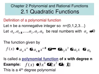
Polynomial Function Degree Example Constant 0 f(x) = 4 Linear 1 f(x) = 3x + 1 Quadratic 2 f(x) = 4x2 x + 9 Cubic 3 f(x) = x3 +2x2 x + 11 Quartic 4 f(x) = x4 3.2x3 + 0.1x Polynomial Function A polynomial functionP is given by where the coefficients an, an - 1, …, a1, a0 are real numbers and the exponents are whole numbers.
Example • Using the leading term-test, match each of the following functions with one of the graphs AD, which follow. a) b) c) d)
Leading Term Degree of Leading Term Sign of Leading Coeff. Graph 3x4 Even Positive D 5x3 Odd Negative B x5 Odd Positive A x6 Even Negative C Solution
Finding Zeros of Factored Polynomial Functions • If c is a real zero of a function (that is, f(c) = 0), then (c, 0) is an x-intercept of the graph of the function. Example: Find the zeros of
Solution: To solve the equation f(x) = 0, we use the principle of zero products, solving x 1 = 0 and x + 2 = 0. The zeros of f(x) are 1 and 2. See graph on right. Finding Zeros of Factored Polynomial Functions continued
Even and Odd Multiplicity If (x c)k, k 1, is a factor of a polynomial function P(x) and: k is odd, then the graph crosses the x-axis at (c, 0); k is even, then the graph is tangent to the x-axis at (c, 0).
Find the real zeros of the function f given by f(x) = 0.2x3 1.1x2 0.3x + 3 Look for points where the graph crosses the x-axis. It appears that there are three zeros, one between 2 and 1, one near 2, and one near 5. We use the ZERO feature to find them. The zeros are approximately x = 1.56689, y = 0 x = 1.82693, y = 0 x = 5.2399, y = 0 Finding Real Zeros on a Calculator
3.2Graphing Polynomial Functions Graph polynomial functions. Use the intermediate value theorem to determine whether a function has a real zero between two given real numbers.
Graphing Polynomial Functions • If P(x) is a polynomial function of degree n, the graph of the function has: at most n real zeros, and thus at most nx-intercepts; at most n 1 turning points. (Turning points on a graph, also called relative maxima and minima, occur when the function changes from decreasing to increasing or from increasing to decreasing.)
Steps to Graph a Polynomial Function 1. Use the leading-term test to determine the end behavior. 2. Find the zeros of the function by solving f(x) = 0. Any real zeros are the first coordinates of the x-intercepts. 3. Use the x-intercepts (zeros) to divide the x-axis into intervals and choose a test point in each interval to determine the sign of all function values in that interval. 4. Find f(0). This gives the y-intercept of the function. 5. If necessary, find additional function values to determine the general shape of the graph and then draw the graph. 6. As a partial check, use the facts that the graph has at most nx-intercepts and at most n 1 turning points. Multiplicity of zeros can also be considered in order to check where the graph crosses or is tangent to the x-axis.
Example Graph the polynomial function f(x) = 2x3 + x2 8x 4. Solution: 1. The leading term is 2x3. The degree, 3, is odd, the coefficient, 2, is positive. Thus the end behavior of the graph will appear as: 2. To find the zero, we solve f(x) = 0. Here we can use factoring by grouping.
Example continued Factor: The zeros are 1/2, 2, and 2. The x-intercepts are (2, 0), (1/2, 0), and (2, 0). 3. The zeros divide the x-axis into four intervals: (, 2), (2, 1/2), (1/2, 2), and (2, ). We choose a test value for x from each interval and find f(x).
Interval Test Value, x Function value, f(x) Sign of f(x) Location of points on graph (, 2) 3 25 Below x-axis (2, 1/2) 1 3 + Above x-axis (1/2, 2) 1 9 Below x-axis (2, ) 3 35 + Above x-axis Example continued 4. To determine the y-intercept, we find f(0): The y-intercept is (0, 4).
x f(x) 2.5 9 1.5 3.5 1.5 7 Example continued 5. We find a few additional points and complete the graph. 6. The degree of f is 3. The graph of f can have at most 3 x-intercepts and at most 2 turning points. It has 3 x-intercepts and 2 turning points. Each zero has a multiplicity of 1; thus the graph crosses the x-axis at 2, 1/2, and 2. The graph has the end behavior described in step (1). The graph appears to be correct.
Intermediate Value Theorem • For any polynomial function P(x) with real coefficients, suppose that for a b, P(a) and P(b) are of opposite signs. Then the function has a real zero between a and b. Example: Using the intermediate value theorem, determine, if possible, whether the function has a real zero between a and b. a) f(x) = x3 + x2 8x; a = 4 b = 1 b) f(x) = x3 + x2 8x; a = 1 b = 3
Solution f(1) = (1)3 + (1)2 8(1) = 6 f(3) = (3)3 + (3)2 8(3) = 12 By the intermediate value theorem, since f(1) and f(3) have opposite signs, then f(x) has a zero between 1 and 3. We find f(a) and f(b) and determine where they differ in sign. The graph of f(x) provides a visual check. f(4) = (4)3 + (4)2 8(4) = 16 f(1) = (1)3 + (1)2 8(1) = 8 By the intermediate value theorem, since f(4) and f(1) have opposite signs, then f(x) has a zero between 4 and 1.
3.3Polynomial Division; The Remainder and Factor Theorems Perform long division with polynomials and determine whether one polynomial is a factor of another. Use synthetic division to divide a polynomial by x c. Use the remainder theorem to find a function value f(c). Use the factor theorem to determine whether x c is a factor of f(x).
Division and Factors • When we divide one polynomial by another, we obtain a quotient and a remainder. If the remainder is 0, then the divisor is a factor of the dividend. Example: Divide to determine whether x + 3 and x 1 are factors of
Division and Factors continued • Divide: Since the remainder is –64, we know that x + 3 is not a factor.
Division and Factors continued • Divide: Since the remainder is 0, we know that x 1 is a factor.
The Remainder Theorem If a number c is substituted for x in a polynomial f(x), then the result f(c) is the remainder that would be obtained by dividing f(x) by x c. That is, if f(x) = (x c)• Q(x) + R, then f(c) = R. Synthetic division is a “collapsed” version of long division; only the coefficients of the terms are written.
2 –4 1 6 2 0 50 –8 –14 –16 –28 –56 –4 –7 –8 –14 –28 –6 Example Use synthetic division to find the quotient and remainder. The quotient is – 4x4 – 7x3 – 8x2 – 14x – 28 and the remainder is –6. Note: We must write a 0 for the missing term.
4 1 –6 11 –6 4 –8 12 1 –2 3 6 Example • Determine whether 4 is a zero of f(x), where f(x) = x3 6x2 + 11x 6. • We use synthetic division and the remainder theorem to find f(4). • Since f(4) 0, the number is not a zero of f(x).
For a polynomial f(x), if f(c) = 0, then x c is a factor of f(x). Example: Let f(x) = x3 7x + 6. Factor f(x) and solve the equation f(x) = 0. Solution: We look for linear factors of the form x c. Let’s try x 1. Since f(1) = 0, we know that x 1 is one factor and the quotient x2 + x 6 is another. So, f(x) = (x 1)(x + 3)(x 2). For f(x) = 0, x = 3, 1, 2. 1 1 0 –7 6 1 1 –6 1 1 –6 0 The Factor Theorem
3.4Theorems about Zeros of Polynomial Functions Find a polynomial with specified zeros. For a polynomial function with integer coefficients, find the rational zeros and the other zeros, if possible. Use Descartes’ rule of signs to find information about the number of real zeros of a polynomial function with real coefficients.
Every polynomial function of degree n, with n 1, has at least one zero in the system of complex numbers. Example: Find a polynomial function of degree 4 having zeros 1, 2, 4i, and 4i. Solution: Such a polynomial has factors (x 1),(x 2), (x 4i), and (x + 4i), so we have: Let an = 1. The Fundamental Theorem of Algebra
Zeros of Polynomial Functions with Real Coefficients • If a complex number a + bi, b 0, is a zero of a polynomial function f(x) with real coefficients, then its conjugate, a bi, is also a zero. (Nonreal zeros occur in conjugate pairs.) • Rational CoefficientsIf where a and b are rational and c is not a perfect square, is a zero of a polynomial function f(x) with rational coefficients, then is also a zero.
Example • Suppose that a polynomial function of degree 6 with rational coefficients has 3 + 2i, 6i, and as three of its zeros. Find the other zeros. Solution: The other zeros are the conjugates of the given zeros, 3 2i, 6i, and There are no other zeros because the polynomial of degree 6 can have at most 6 zeros.
Rational Zeros Theorem • Let where all the coefficients are integers. Consider a rational number denoted by p/q, where p and q are relatively prime (having no common factor besides 1 and 1). If p/q is a zero of P(x), then p is a factor of a0 and q is a factor of an.
Example • Given f(x) = 2x3 3x2 11x + 6: a) Find the rational zeros and then the other zeros. b) Factor f(x) into linear factors. Solution: a) Because the degree of f(x) is 3, there are at most 3 distinct zeros. The possibilities for p/q are:
–1 1 2 2 –3 –3 –11 –11 6 6 2 –2 –1 5 –12 6 2 2 –1 –5 –12 –6 –6 12 Example continued • Use synthetic division to help determine the zeros. It is easier to consider the integers before the fractions. We try 1: We try 1: Since f(1) = 6, 1 is not a zero.Since f(1) = 12, 1 is not zero.
3 2 –3 –11 6 6 9 –6 2 3 –2 0 Example continued • We try 3: . We can further factor 2x2 + 3x 2 as (2x 1)(x + 2). Since f(3) = 0, 3 is a zero. Thus x 3 is a factor. Using the results of the division above, we can express f(x) as
Example continued • The rational zeros are 2, 3 and • The complete factorization of f(x) is:
Descartes’ Rule of Signs Let P(x) be a polynomial function with real coefficients and a nonzero constant term. The number of positive real zeros of P(x) is either: 1. The same as the number of variations of sign in P(x), or 2. Less than the number of variations of sign in P(x) by a positive even integer. The number of negative real zeros of P(x) is either: 3. The same as the number of variations of sign in P(x), or 4. Less than the number of variations of sign in P(x) by a positive even integer. A zero of multiplicity m must be counted m times.
Example • What does Descartes’ rule of signs tell us about the number of positive real zeros and the number of negative real zeros? There are two variations of sign, so there are either two or zero positive real zeros to the equation.
Example continued The number of negative real zeros is either two or zero. Total Number of Zeros 4 Positive 2 2 0 0 Negative 2 0 2 0 Nonreal 0 2 2 4
3.5Rational Functions For a rational function, find the domain and graph the function, identifying all of the asymptotes. Solve applied problems involving rational functions.
Rational Function • A rational function is a function f that is a quotient of two polynomials, that is, where p(x) and q(x) are polynomials and where q(x) is not the zero polynomial. The domain of f consists of all inputs x for which q(x) 0.
Consider . Find the domain and graph f. Solution: When the denominator x + 4 = 0, we have x = 4, so the only input that results in a denominator of 0 is 4. Thus the domain is {x|x 4} or (, 4) (4, ). The graph of the function is the graph of y = 1/x translated to the left 4 units. Example
Vertical Asymptotes • The vertical asymptotes of a rational function f(x) = p(x)/q(x) are found by determining the zeros of q(x) that are not also zeros of p(x). If p(x) and q(x) are polynomials with no common factors other than constants, we need to determine only the zeros of the denominator q(x). • If a is a zero of the denominator, then the line x = a is a vertical asymptote for the graph of the function.
Determine the vertical asymptotes of the function. Factor to find the zeros of the denominator: x2 4 = (x + 2)(x 2) Thus the vertical asymptotes are the lines x = 2 and x = 2. Example