Download

1 / 24
240 likes | 376 Views
Please turn off cell phones, pagers, etc. The lecture will begin shortly. Lecture 20. This lecture will introduce topics from Chapter 12. 2 × 2 frequency tables (Section 12.1). 2. Probability and odds (Section 12.2). 3. Measures of association in 2×2 tables (Section 12.2).

E N D
Please turn off cell phones, pagers, etc. The lecture will begin shortly.
Lecture 20 This lecture will introduce topics from Chapter 12. • 2 × 2 frequency tables (Section 12.1) 2. Probability and odds (Section 12.2) 3. Measures of association in 2×2 tables (Section 12.2)
1. 2 × 2 frequency tables In Chapters 10-11, we learned how to describe relationships among continuous variables: • scatterplots • correlation coefficients • regression analysis Now we begin to examine relationships between categorical variables. More specifically, we’ll consider relationships between variables that are binary.
What is a binary variable? A binary variable is a measurement that has only two possible outcomes. These are also known as dichotomous variables. Examples: • sex (male or female) • treatment in a two-armed experiment • (e.g. aspirin or placebo) • whether a subject has a trait or condition • (e.g. cancer or no cancer) • survival after a specified period of time • (alive or dead)
Freq Yes 10 No 6 Total 16 Frequency table for a binary variable Suppose we take a sample of n subjects and record a binary variable for each subject. For example: Ask 16 students, “Are you registered to vote?” Y Y N Y Y N Y Y N N Y Y Y N N Y A frequency table (or contingency table) records the number of subjects in each category:
Freq Yes 10 No 6 Total 16 Proportions and percentages Once you have the frequency table, you can compute the proportions and percentages in each category by dividing the frequencies by the sample size. Registered: Proportion = 10/16 = 0.625 Percentage = 0.625 × 100 = 62.5% Unregistered: Proportion = 6/16 = 0.375 Percentage = 0.375 × 100 = 37.5%
Sex Registered? Subject 1 M N 2 M N 3 F Y 4 M Y 5 F Y 6 F N 7 M N 8 F N 9 F Y Registered? 10 F Y Yes No 11 M Y 12 F Y Male 4 4 13 M Y Female 6 2 14 M N 15 F Y 16 M Y Two binary variables Suppose that you now have two binary variables for each subject. The 2×2 frequency table (also known as 2×2 contingency table) records the number of subjects in each of the four possible categories.
Heart attack? Yes No Aspirin Placebo Aspirin 104 10,933 Heart attack 104 189 Placebo 189 10,845 No attack 10,933 10,845 Rows and columns When creating a 2×2 table, it’s customary to make the • rows correspond to the explanatory variable • columns correspond to the response variable Wrong: Right:
Heart attack? Yes No Total Aspirin 104 10,933 104 + 10,933 Placebo 189 10,845 189 + 10,845 Total 11,037 + 11,034 104 + 189 10,933 + 10,845 Margins We often add an extra row and column to hold the row and column totals. These are called the margins. 11,037 11,034 293 21,778 22,071 or 293 + 21,778 (Grand total or sample size n)
Heart attack? Yes No Total Aspirin 104 10,933 11,037 Placebo 189 10,845 11,034 Total 293 21,778 22,071 Proportion with heart attack Row proportions To uncover the relationship between the explanatory (row) variable and response (column) variable, compute the row proportions and percentages: • choose one of the first two columns • divide by the third column Aspirin 104 / 11,037 = .0094 Placebo 189 / 11,034 = .0171
Rate of heart attack proportion % per 1,000 Aspirin .0094 Placebo .0171 Percentages and rates When the row proportions are small, it is customary to express them as percentages, rates per 1,000, per 10,000, per 100,000, etc. • proportion × 100 = percent • proportion × 1,000 = rate per 1,000 • proportion × 10,000 = rate per 10,000 0.94 9.4 1.71 17.1
0 1 2. Probability and odds Probability is a number between 0 and 1 that indicates how likely it is that an event will occur unlikely likely probability = 0 means that the event will never occur probability = 1 means that the event will always occur probability = 0.5 means that the event is just as likely to occur as not Values close to zero indicate that the event is unlikely; values close to one indicate that it is likely.
to ∞ 0 1 Odds Another measure of how likely an event is to occur is odds. Odds ranges from 0 to ∞. unlikely likely odds = 0 means that the event will never occur odds = ∞ means that the event will always occur odds = 1 (often written as 1:1, which is the same as 1/1) means that the event is just as likely to occur as not odds = 2 (often written as 2:1, which is the same as 2/1) means that the event is twice as likely to occur as not
Odds as ratios Gamblers sometimes express odds as a ratio a:b where b is something other than 1. For example, they may say “the odds are 3:2.” Note that odds of 3:2 are the same as 3/2 = 1.5 So if you ever see odds expressed as a:b, you should divide a by b to re-express the odds as a number between 0 and ∞.
probability 0 .25 .5 .667 .75 .8 1 odds 0 1 2 3 4 Prob = 0 corresponds to odds = 0 Prob = .25 corresponds to odds = 0.333 Prob = .50 corresponds to odds = 1 Prob = .667 corresponds to odds = 2 Prob = .75 corresponds to odds = 3 Prob = .8 corresponds to odds = 4 Odds and probability Odds and probability are not the same!
probability odds = 1 - probability Converting probability to odds Given a probability, you can find the odds by the formula Examples Prob = .5 corresponds to odds = .5 /.5 = 1 Prob = .7 corresponds to odds = .7 / .3 = 2.33 Prob = .9 corresponds to odds = .9 / .1 = 9 Prob = .99 corresponds to odds = .99 / .01 = 99
odds probability = 1 + odds Converting odds to probability Given a probability, you can find the odds by the formula Examples odds = .5 corresponds to prob = .5/1.5 = 0.333 odds = 3 corresponds to prob = 3/4 = 0.75 odds = 10 corresponds to prob = 10/11 = 0.909 odds = 25 corresponds to prob = 25/26 = 0.962
Rare events For rare events (probabilities close to zero), odds and probabilities are nearly the same. Examples Prob = .001 corresponds to odds = .001001 Prob = .01 corresponds to odds = .0101 Prob = .02 corresponds to odds = .0204 Prob = .03 corresponds to odds = .0309 When discussing rare events, the distinction between odds and probability is often unimportant.
# of subjects having the trait Sample proportion = # of subjects in the sample Freq Yes 10 No 6 Total 16 Estimating probabilities from frequency tables The sample proportion is an estimate of the probability that a subject chosen at random from the population has the trait. Example “Are you registered to vote?” The proportion registered is 10/16 = .625 The proportion not registered is 6/16 = .375
# of subjects having the trait Sample odds = # of subjects not having the trait Freq Yes 10 No 6 Total 16 Estimating odds from frequency tables The sample odds is an estimate of the odds that a subject chosen at random from the population has the trait. Example The estimated odds of being registered is 10/6 = 1.67 The estimated odds of not being registered is 6/10 = 0.6
3. Measures of association in 2×2 tables Recall that with two continuous variables, a useful measure of association is the correlation coefficient. For two binary variables, the most common measures of association are • Relative risk • Odds ratio The relative risk is a ratio of proportions. The odds ratio is a ratio of odds.
Heart attack? Yes No Total Aspirin 104 10,933 11,037 Placebo 189 10,845 11,034 Total Proportion with heart attack 293 21,778 22,071 Aspirin 104 / 11,037 = .0094 Placebo 189 / 11,034 = .0171 Estimating the relative risk • Compute the proportions for each row • Divide one proportion by the other Example The estimated relative risk is .0094 / .0171 = 0.55
Heart attack? Yes No Total Aspirin 104 10,933 11,037 Placebo 189 10,845 11,034 Total 293 21,778 22,071 Estimated odds of heart attack Aspirin 104 / 10,933 = .0095 Placebo 189 / 10,845 = .0174 Computing the odds ratio • Compute the odds for each row • Divide one odds by the other Example The estimated odds ratio is .0095 / .0174 = 0.55
a b c d Heart attack? Yes No Total The estimated odds ratio is 104 × 10,845 Aspirin 104 10,933 11,037 = 0.55 Placebo 189 10,845 11,034 10,933 × 189 Total 293 21,778 22,071 Easier way to estimate the odds ratio If the frequencies in the 2×2 table are then the estimated odds ratio is (a×d) / (b×d). Example