NASA Biodiversity and Ecological Forecasting Team Meeting 29 – 31 August 2005 Washington, DC Fig.2

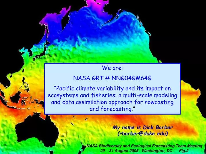
1. We are: NASA GRT # NNG04GM64G “Pacific climate variability and its impact on ecosystems and fisheries: a multi-scale modeling and data assimilation approach for nowcasting and forecasting.” My name is Dick Barber (rbarber@duke.edu) NASA Biodiversity and Ecological Forecasting Team Meeting 29 – 31 August 2005 Washington, DC Fig.2

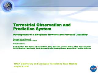
2. Dick Barber – Duke University Fei Chai - University of Maine Yi Chao - Jet Propulsion Lab of Cal Tech Francisco Chavez - Monterey Bay Aquarium Research Institute Joaquim Goes - Bigelow Laboratory for Ocean Sciences Michael Alexander - NOAA Climate Diagnostics Center NASA Biodiversity and Ecological Forecasting Team Meeting 29 – 31 August 2005 Washington, DC Fig. 3

3. Goal: Deliver forecasts of circulation and ecosystem function in the Pacific Ocean which can force fish population models to make forecasts of fish abundance with 6 to 9 months lead-time. NASA Biodiversity and Ecological Forecasting Team Meeting 29 – 31 August 2005 Washington, DC Fig.4

4. 30 years ago (1975) we had an NSF project, Coastal Upwelling Ecosystems Analysis (CUEA), based on the premise that: “Prediction of the response of the coastal upwelling ecosystem to natural variations, man-made environmental perturbations or to different harvesting strategies is possible from knowledge of a few biological, physical and meteorological variables...” NASA Biodiversity and Ecological Forecasting Team Meeting 29 – 31 August 2005 Washington, DC

5. “The goal of the Coastal Upwelling Ecosystems Analysis Program is to understand the coastal upwelling ecosystem well enough to predict its response far enough in advance to be useful to mankind.” Written in May 1975 Little did we know………… NASA Biodiversity and Ecological Forecasting Team Meeting 29 – 31 August 2005 Washington, DC

6. CUEA was successful by NSF’s basic research criteria, butthe goal was never achieved …... • the technology, vision and science of 30 years ago was simply inadequate: • - undersampling in time and space • - omission of remote forcing in the CU paradigm • complete unawareness of decadal variability - over-simplified linear food web theory • - limited to 2D and uncoupled modeling NASA Biodiversity and Ecological Forecasting Team Meeting 29 – 31 August 2005 Washington, DC

7. 1. Two conceptual advances in ocean ecological theory: 1a. two-path food web (need for picophytoplankton and micrograzers) 1b. role of Fe in ocean ecosystems NASA Biodiversity and Ecological Forecasting Team Meeting 29 – 31 August 2005 Washington, DC

8. What has changed ? The ecology of 1975 was pretty good, only two conceptual advances in ocean ecological theory: 1a. two-path food web (need for picophytoplankton and micrograzers) 1b. role of Fe in ocean ecosystems NASA Biodiversity and Ecological Forecasting Team Meeting 29 – 31 August 2005 Washington, DC

9. NASA Biodiversity and Ecological Forecasting Team Meeting 29 – 31 August 2005 Washington, DC

10. But the big change is: 2.A revolution in observing systems inmode, resolution & quantity. 3.An even more profound revolution in computational power. NASA Biodiversity and Ecological Forecasting Team Meeting 29 – 31 August 2005 Washington, DC

11. 2.The observational revolution (satellites and moorings) gives continuous access to the time and space scales of variability forcing ocean ecosystems. NASA Biodiversity and Ecological Forecasting Team Meeting 29 – 31 August 2005 Washington, DC

12. 3.The computational revolution makes possible and enormous increases in both time and space resolution (physical) and model complexity (ecology). NASA Biodiversity and Ecological Forecasting Team Meeting 29 – 31 August 2005 Washington, DC

13. Project Columbia and ROMS at NASA Ames 12.5-km Computer at NASA Advanced Supercomputing Facility: 20 interconnected SGI® Altix® 512-processor systems a total of 10,240 Intel Itanium 2 processors Pacific basin-scale ROMS: (1520x1088x30) 12.5-km horizontal resolutions & 30 vertical layers 50-year (1950-2000) integration NASA Biodiversity and Ecological Forecasting Team Meeting 29 – 31 August 2005 Washington, DC

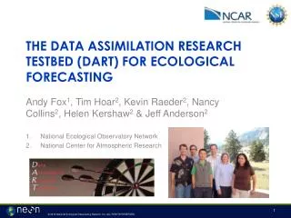
14. …that is, NASA satellites and computational-power enable us to: observe the ocean (earth) continuously, initialize andassimilate the observations into models with the time/space resolution and complexity needed for accurate ecosystem and fisheries forecasts. NASA Biodiversity and Ecological Forecasting Team Meeting 29 – 31 August 2005 Washington, DC

15. Internal/intrinsic variability Features (<10 km, days) Model resolution (~1 km, hours) Observation 2.5-km 5-km 10-km 20-km Scale convergence of eddy kinetic energy of model and observationsin a coastal upwelling system Eddy kinetic energy (cm2s-2) Drifter Model Resolution (km) NASA Biodiversity and Ecological Forecasting Team Meeting 29 – 31 August 2005 Washington, DC

16. xf 1-week forecast Xa = xf + xf Weekly assimilation cycle Xa Initial condition analysis Week 5 Week 4 Week 2 Week 3 Week 1 Assimilation and Initialization 3-dimensional variational (3DVAR) method: y: observation x: model J = 0.5 (x-xf)T B-1 (x-xf) + 0.5 (h x-y)T R-1 (h x-y)

17. Now, for a look at the Peru coastal upwelling ecosystem: Time series: 1955 – 2005 Anchovy catch by the Peruvian fishery Temperature anomaly (°C) in Niño 1 and 2 regions (3-month running mean of monthly SST anomalies) Niño 2 Niño 1 NASA Biodiversity and Ecological Forecasting Team Meeting 29 – 31 August 2005 Washington, DC

18. NASA Biodiversity and Ecological Forecasting Team Meeting 29 – 31 August 2005 Washington, DC

19. Natural interannual (ENSO) and decadal (PDO, NAO)climate variability, together with fishing itself, drive large variations in fish stocks. • Inability to account for externally-driven variability in fish stocks prevents successful management. • Tools are now available to incorporate climate effects into ecosystem-based management models. • Lead time is needed for economic usefulness. • Operational 6 to 9 month physical forecasts(for the Pacific) are now available.

20. Show movie. NASA Biodiversity and Ecological Forecasting Team Meeting 29 – 31 August 2005 Washington, DC

21. We have: • Improved food web theory (Fe and 2-path) • Realistic and validated physical and food web models • Observing tools, satellites, moorings, TOGA-TAO, etc. for initialization and assimilation • 4. Computational power needed for scale convergence, fine time steps and many model compartments • 5. Operational 6 and 9 month ENSO forecasts NASA Biodiversity and Ecological Forecasting Team Meeting 29 – 31 August 2005 Washington, DC

22. Summary: The capability exists to deliver operational marine ecosystem forecasts with enough lead time, accuracy and precision to be socially and economically beneficial. NASA Biodiversity and Ecological Forecasting Team Meeting 29 – 31 August 2005 Washington, DC