Download

1 / 30
360 likes | 641 Views
C4.5 and CHAID Algorithm. Pavan J Joshi 2010MCS2095 Special Topics in Database Systems. Outline. Disadvantages of ID3 algorithm C4.5 algorithm Gain ratio Noisy Data and overfitting Tree pruning Handling of missing values Error estimation Continuous data CHAID. ID3 Algorithm.

E N D
C4.5 and CHAID Algorithm Pavan J Joshi 2010MCS2095 Special Topics in Database Systems
Outline • Disadvantages of ID3 algorithm • C4.5 algorithm • Gain ratio • Noisy Data and overfitting • Tree pruning • Handling of missing values • Error estimation • Continuous data • CHAID
ID3 Algorithm • Top down construction of decision tree by recursively selecting the “best attribute” to use at the current node, based on the training data • It can only deal with nominal data • It is not robust in dealing with noisy data sets • It overfits the tree to the training data • It creates unnecessarily complex trees without pruning • It does not handle missing data values well
C4.5 Algorithm • An Improvement over ID3 algorithm • Designed to handle • Noisy data better • Missing data • Pre and post pruning of decision trees • Attributes with continuous values • Rule Derivation
Using Gain Ratios • The notion of Gain introduced earlier favors attributes that have a large number of values. • If we have an attribute D that has a distinct value for each record, then Info(D,T) is 0, thus Gain(D,T) is maximal. • To compensate for this Quinlan suggests using the following ratio instead of Gain: GainRatio(D,T) = Gain(D,T) / SplitInfo(D,T) • SplitInfo(D,T) is the information due to the split of T on the basis of value of categorical attribute D. SplitInfo(D,T) = I(|T1|/|T|, |T2|/|T|, .., |Tm|/|T|) where {T1, T2, .. Tm} is the partition of T induced by value of D.
Noisy data • Many kinds of "noise" that could occur in the examples: • Two examples have same attribute/value pairs, but different classifications • Some values of attributes are incorrect because of: • Errors in the data acquisition process • Errors in the preprocessing phase • The classification is wrong (e.g., + instead of -) because of some error • Some attributes are irrelevant to the decision-making process, • e.g., color of a die is irrelevant to its outcome. • Irrelevant attributes can result in overfitting the training data.
What’s Overfitting? • Overfitting =Given a hypothesis space H, a hypothesis hєH is said to overfitthe training data if there exists some alternative hypothesis h’єH, such that 1. h has smaller error than h’ over the training examples, but 2. h’ has a smaller error than h over the entire distribution of instances.
Why Does my Method Overfit ? • In domains with noise or uncertainty the system may try to decrease the training error by completely fitting all the training examples
Fix overfitting/overlearning problem Ok, my system may overfit… Can I avoid it? • Yes! Do not include branches that fit data too specifically How? 1. Pre-prune: Stop growing a branch when information becomes unreliable 2. Post-prune: Take a fully-grown decision tree and discard unreliable parts
Pre - Pruning • Based on statistical significance test • Stop growing the tree when there is no statistically significant association between any attribute and the class at a particular node • Use all available data for training and apply the statistical test to estimate whether expanding/pruning a node is to produce an improvement beyond the training set • Most popular test: chi-squared test • chi2 = sum( (O-E)2/ E ) Where, O = observed data, E = expected values based on hypothesis.
Example • Example : 5 schools have the same test. Total score is 375, individual results are: 50, 93, 67, 78 and 87. Is this distribution significant, or was it just luck? Average is 75. (50-75)2/75 + (93-75)2/75 + (67-75)2/75 + (78-75)2/75 +(87-75)2/75 = 15.55 This distribution is significant !
Post – pruning • Two pruning operations: 1. Subtree replacement 2. Subtree raising
Color Color FAILURE red blue red blue 2 success 4 failure 1 success 1 failure 1 success 3 failure 0 success 1 failure 1 success 0 failure Subtree Replacement • Pruning of the decision tree is done by replacing a whole subtree by a leaf node. • The replacement takes place if a decision rule establishes that the expected error rate in the subtree is greater than in the single leaf. • E.g., • Training: eg, one training red success and one training blue Failures • Test: three red failures and one blue success • Consider replacing this subtree by a single Failure node. • After replacement we will have only two errors instead of five failures.
Error Estimation • Error estimate of a subtree is a weighted sum of error estimates of all its leaves • Error estimation at every node • Z is a constant 0.69 • F is the error on the training data • N is the number of instances covered by the leaf
Deal with continuous data • When dealing with nominal data, We evaluated the grain for each possible value • In continuous data, we have infinite values. What should we do? • Continuous-valued attributes may take infinite values, but we have a limited number of values in our instances (at most N if we have N instances) • Therefore, simulate that you have N nominal values • Evaluate information gain for every possible split point of the Attribute Choose the best split point • The information gain of the attribute is the information gain of the best split
Split in continuous data • Split on temperature attribute • For example, in the above array of values the split is occurring between 71 and 72( N distinct values meaning at most N-1 splits) • The threshold value is the largest value from the whole training set which lies between 71 and 72 • Of all such splits , the one with the best Information Gain is chosen for the node
Deal with missing values • Many possible approaches • Treat them as different values • Propogatethe cases containing such values down the tree without considering them in the “Information Gain” calculation
From Trees to Rules • Now we've built a tree, it might be desirable to re-express it as a list of rules. • Simple Method: Generate a rule by conjunction of tests in each path through the tree. • Eg: if temp > 71.5 and ... and windy = false then play=yes if temp > 71.5 and ... and windy = true then play=no • But these rules are more complicated than necessary. • Instead we could use the pruning method of C4.5 to prune rules as well as trees.
Rule Derivation for each rule, e = error rate of rule e' = error rate of rule - finalCondition if e' < e, rule = rule-finalCondition recurse remove duplicate rules • Expensive: Need to reevaluate entire training set for every condition! • Might create duplicate rules if all of the final conditions from a path are removed.
Chi-Squared Automatic Interaction Detection(CHAID) • It is one of the oldest tree classification methods originally proposed by Kass in 1980 • The first step is to create categorical predictors out of any continuous predictors by dividing the respective continuous distributions into a number of categories with an approximately equal number of observations • The next step is to cycle through the predictors to determine for each predictor the pair of (predictor) categories that is least significantly different with respect to the dependent variable • The next step is to choose the split the predictor variable with the smallest adjusted p-value, i.e., the predictor variable that will yield the most significant split • Continue this process until no further splits can be performed
Algorithm Dividing the cases that reach a certain node in the tree 1. Cross tabulate the response variable (target) with each of the explanatory variables.
Algorithm – step 2 2. When there are more than two columns, find the "best" subtable formed by combining column categories 2.1 This is applied to each table with more than 2 columns. 2.2 Compute Pearson X2 tests for independence for each allowable subtable 2.3 Look for the smallest X2value. If it is not significant, combine the column categories. 2.4 Repeat step 2 if the new table has more than two columns
Algorithm – step 3 3 Allows categories combined at step 2 to be broken apart. 3.1 For each compound category consisting of at least 3 of the original categories, find the “most significant" binary split 3.2 if X2 is significant, implement the split and return to step 2. 3.3 otherwise retain the compound categories for this variable, and move on to the next variable
Algorithm - Step 4 4. You have now completed the “optimal” combining of categories for each explanatory variable. 4.1 Find the most significant of these “optimally” merged explanatory variables 4.2 Compute a “Bonferroni” adjusted chi-squared test of independence for the reduced table for each explanatory variable.
Algorithm – Step 5 5 Use the “most significant" variable in step 4 to split the node with respect to the merged categories for that variable. 5.1repeat steps 1-5 for each of the offspring nodes. 5.2Stop if • no variable is significant in step 4. • the number of cases reaching a node is below a specified limit.
References • C4.5 Algorithm and Multivariate decision trees by Thales senhKorting • http://www.statsoft.com/textbook/chaid-analysis/ • http://www.public.iastate.edu/~kkoehler/stat557/tree14p.pdf