Download
1 / 62
630 likes | 786 Views
Solar Convection Simulations. Robert Stein, David Benson - Mich. State Univ. Aake Nordlund - Niels Bohr Institute. Movie by Mats Carlsson. METHOD. Solve conservation equations for: mass, momentum, internal energy & induction equation. Conservation Equations. Mass.

E N D
Solar Convection Simulations Robert Stein, David Benson - Mich. State Univ. Aake Nordlund - Niels Bohr Institute
Movie by Mats Carlsson
METHOD • Solve conservation equations for: mass, momentum, internal energy & induction equation
Conservation Equations Mass Momentum Energy Magnetic Flux
Numerical Method • Spatial differencing • 6th-order staggered finite difference,3 points either side • Spatial interpolation • 5th order, staggered • Time advancement • 3rd order Runga-Kutta
Radiation Heating/Cooling • LTE • Non-gray, 4 bin multi-group • Formal Solution Calculate J - B by integrating Feautrier equations along one vertical and 4 slanted rays through each grid point on the surface. • Produces low entropy plasma whose buoyancy work drives convection
5 Rays Through Each Surface Grid Point Interpolate source function to rays at each height
Equation of State • Tabular EOS includes ionization, excitationH, He, H2, other abundant elements
Boundary Conditions • Current: ghost zones loaded by extrapolation • Density, top hydrostatic, bottom logarithmic • Velocity, symmetric • Energy (per unit mass), top = slowly evolving average • Magnetic (Electric field), top -> potential, bottom -> fixed value in inflows, damped in outflows • Future: ghost zones loaded from characteristics normal to boundary(Poinsot & Lele, JCP, 101, 104-129, 1992)modified for real gases
t Z Fluid Parcelsreaching the surface Radiate away their Energy and Entropy r Q E S
3-D simulations (Stein & Nordlund) v ~ k-1/3 MDI correlation tracking (Shine) MDI doppler (Hathaway) TRACE correlation tracking (Shine) v ~ k Solar velocity spectrum
Line Profiles observed simulation Line profile without velocities. Line profile with velocities.
Convection produces line shifts, changes in line widths. No microturbulence, macroturbulence. Average profile is combination of lines of different shifts & widths. average profile
P-Mode Excitation Triangles = simulation, Squares = observations (l=0-3) Excitation decreases both at low and high frequencies
Initialization • Start from existing 12 x 12 x 9 Mm simulation • Extend adiabatically in depth to 20 Mm,no fluctuations in extended portion, relax for a solar day to develop structure in extended region • Double horizontally + small fraction of stretched fluctuations to remove symmetry,relax to develop large scale structures • Currently: 48x48x20 Mm100 km horizontal, 12-75 km vertical resolution
Initialization Double horizontally + small fraction stretched : Uz at 0.25 Mm Snapshots of methods + composite (?)
Initialization Double horizontally + small fraction stretched : Uz at 17.3 Mm
Mean Atmosphere Temperature, Density and Pressure (K) (105 dynes/cm2) (10-7 gm/cm2)
Mean Atmosphere Ionization of He, He I and He II
Energy Fluxes ionizationenergy 3X larger energy than thermal
Unipolar Field • Impose uniform vertical field on snapshot of hydrodynamic convection • Boundary Conditions: B -> potential at top, B vertical at bottom • B rapidly swept into intergranular lanes
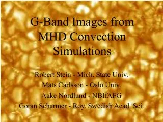
G-bandimages from simulationat disk center & towards limb(by Mats Carlsson) Notice: Hilly appearance of granules Striated bright walls of granules Micropore at top center Dark bands moving across granules
Comparison with observations Observation, mu=0.63 Simulation, mu=0.6
Center to Limb Movie by Mats Carlsson
G-band & Magnetic Field Contours: .5, 1, 1.5 kG (gray) 20 G (red/green)
Magnetic concentrations: cool, low r,low opacity.Towards limb,radiation emerges from hot granulewalls behind.On optical depth scale,magneticconcentrations are hot, contrast increases with opacity
Magnetic Field &VelocityHigh velocity sheets at edges of flux concentration
G-bandimages from simulationat disk center & towards limb(by Mats Carlsson) Notice: Dark bands moving across granules