Download
1 / 31
330 likes | 501 Views
Computability Julia sets. Mark Braverman Microsoft Research January 6, 2009. Julia Sets. Focus on the quadratic family. Let c be a complex parameter. Consider the following discrete-time dynamical system on the complex plane: z ↦ z 2 + c

E N D
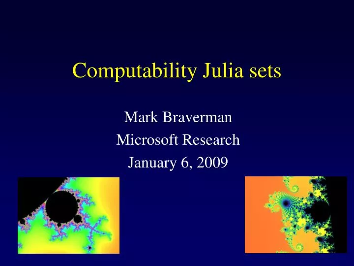
Computability Julia sets Mark Braverman Microsoft Research January 6, 2009
Julia Sets • Focus on the quadratic family. • Let c be a complex parameter. • Consider the following discrete-time dynamical system on the complex plane: z ↦z2 + c • The simplest non-trivial polynomial dynamical system on the complex plane.
The Julia set • The filled Julia set Kc is the set of initial z’s for which the orbit does not escape to ∞. • The Julia set Jc is the boundary of Kc: Jc =∂Kc. • Jc is also the set of points around which the dynamics is unstable.
Example: c = -0.12 + 0.665 i z ↦z2 + c
Iterating z ↦ z2 - 0.12 + 0.665 i z ↦z2 + c
Iterating z ↦ z2 - 0.12 + 0.665 i z ↦z2 + c
Iterating z ↦ z2 - 0.12 + 0.665 i z ↦z2 + c
Iterating z ↦ z2 - 0.12 + 0.665 i z ↦z2 + c
Iterating z ↦ z2 - 0.12 + 0.665 i z ↦z2 + c
Iterating z ↦ z2 - 0.12 + 0.665 i z ↦z2 + c
The Julia set • The filled Julia set Kc is the set of initial z’s for which the orbit does not escape to ∞. • The Julia set Jc is the boundary of Kc: Jc = ∂Kc. • Jc is also the set of points around which the dynamics is unstable.
Iterating z ↦ z2- 0.391 - 0.587 i z ↦z2 + c
Iterating z ↦ z2- 0.391 - 0.587 i z ↦z2 + c “rotation” by an angle θ
Computing Kc and Jc • Given the parameter c as an input, compute Kc and Jc. • The parameter c describes the rule of the dynamics – “its world”.
Jc c = −0.46768… + 0.56598…i Computability model • We use the “bit-computability” notion, which accounts for the cost of the operations on a Turing Machine. • Dates back to [Turing36], [BanachMazur37]. TM
Input – giving c to TM • The input c is given by an oracle φ(m). • On query m the oracle outputs a rational approximation of c within an error of 2-m. • TM is allowed to query c with any finite precision. c = −0.46768… + 0.56598…i TM
φ(2) = −0.4+0.5 i Input – giving c to TM • The input c is given by an oracle φ(m). • On query m the oracle outputs a rational approximation of c within an error of 2-m. • TM is allowed to query c with any finite precision. c = −0.46768… + 0.56598…i φ(m) m=2 TM
φ(10) = −0.468+0.566 i Input – giving c to TM • The input c is given by an oracle φ(m). • On query m the oracle outputs a rational approximation of c within an error of 2-m. • TM is allowed to query c with any finite precision. c = −0.46768… + 0.56598…i φ(m) m=10 TM
φ(7) = −0.466+0.567 i Input – giving c to TM • The input c is given by an oracle φ(m). • On query m the oracle outputs a rational approximation of c within an error of 2-m. • TM is allowed to query c with any finite precision. c = −0.46768… + 0.56598…i φ(m) m=7 TM
Output • Given a precision parameter n, TM needs to output a 2-n-approximation of Jc, which is a “picture” of the set. Jc φ(m) TM
Output • A 2-n-approximation of Jc, is made of pixels of size ≈2-n. • For each pixel, need to decide whether to paint it white or black. Jc
Coloring a Pixel No Yes ??? • We use round pixels – equivalent up to a constant. • A pixel is a circle of radius 2-nwith a rational center. • Put it in if it intersects Jc. • If twice the pixel does not intersect Jc, leave it out. • Otherwise, don’t care. Jc
Summary ?
Theorem [BY07]: There is an algorithm A that computes a number c such that no machine with access to c can compute Jc. In fact, computing Jc is as hard as solving the Halting Problem. • Under a reasonable conjecture from Complex Dynamics, c can be made poly-time computable. Jc A ? c TM
Proving the non-computability theorem • Consider the family z ↦ z2 + e2πiθ z. • When is there a Siegel disc? • Theorem [Brjuno’65]: When the function converges.
Geometric Meaning of Φ(θ) • r(θ) is a measure on the size of the Siegel disc. • r(θ) can be computed from Jc and vice versa. • Theorem[Yoccoz’88], [Buff,Cheritat’03]: The function Φ(θ) + log r(θ) is continuous. • In particular, when Φ(θ)=∞, r(θ)=0. • Theorem[BY’07]: There is an explicit poly-time algorithm that generates a θsuch that Φ(θ) is as hard to compute as the Halting Problem.
Algebraic Geometric Jc A ? c such that Jc has a Siegel disc the rotation angle 2πθ of the Siegel disc r(θ) – the “size” of the Siegel Disc Continuous: heavy machinery [Yoccoz’88], [Buff,Cheritat’03].
Summary ?
disconnected; poly-time connected; poly-time poly-time Non-computable The map of parameters c
Thank You Computability of Julia Sets, M. Braverman and M. Yampolsky. Springer, 2008.