Download
1 / 28
280 likes | 361 Views
Spatial and Temporal Trends in Tidal Flat Shape in San Francisco Bay. Josh Bearman, Carl Friedrichs , Bruce Jaffe, Amy Foxgrover. Main Points. 1) On tidal flats, sediment (especially mud) moves away from high concentration areas and towards areas of weaker energy.

E N D
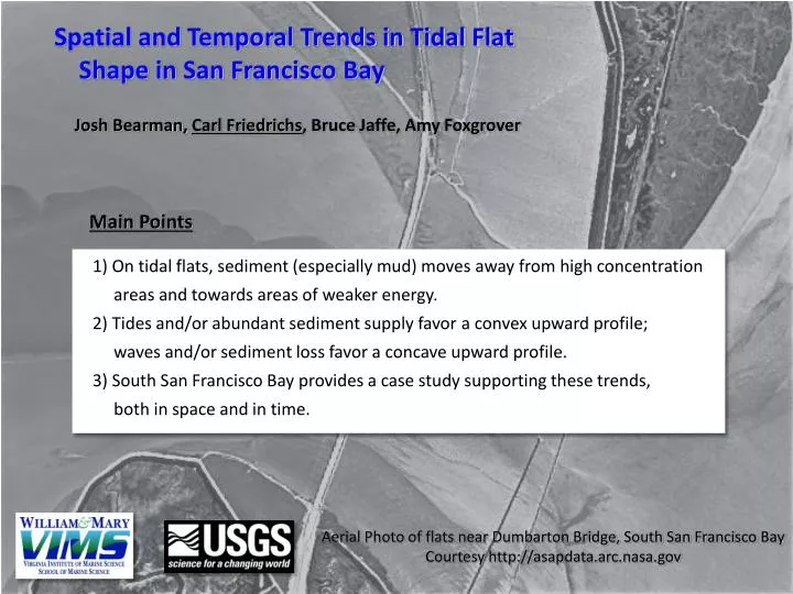
Spatial and Temporal Trends in Tidal Flat Shape in San Francisco Bay Josh Bearman, Carl Friedrichs, Bruce Jaffe, Amy Foxgrover Main Points 1) On tidal flats, sediment (especially mud) moves away from high concentration areas and towards areas of weaker energy. 2) Tides and/or abundant sediment supply favor a convex upward profile; waves and/or sediment loss favor a concave upward profile. 3) South San Francisco Bay provides a case study supporting these trends, both in space and in time. Aerial Photo of flats near Dumbarton Bridge, South San Francisco Bay Courtesy http://asapdata.arc.nasa.gov
Spatial and Temporal Trends in Tidal Flat Shape in San Francisco Bay Josh Bearman, Carl Friedrichs, Bruce Jaffe, Amy Foxgrover Visit Josh at TheHotSeats.net Main Points 1) On tidal flats, sediment (especially mud) moves away from high concentration areas and towards areas of weaker energy. 2) Tides and/or abundant sediment supply favor a convex upward profile; waves and/or sediment loss favor a concave upward profile. 3) South San Francisco Bay provides a case study supporting these trends, both in space and in time. Aerial Photo of flats near Dumbarton Bridge, South San Francisco Bay Courtesy http://asapdata.arc.nasa.gov
South Bay Salt Pond Project • First ponds leveed in 1854 • Currently 26,000 acres of salt ponds in South Bay • October, 2000 • 61% of ponds sold to large conglomerate of GOs, NGOs, private foundations.
What moves sediment across flats? Ans: Tides plus concentration gradients; (i) Due to energy gradients: Tidal advection High energy waves and/or tides Low energy waves and/or tides Higher sediment concentration Tidal advection High energy waves and/or tides Low energy waves and/or tides Lower sediment concentration 1
What moves sediment across flats? Ans: Tides plus concentration gradients; (ii) Due to sediment supply: Tidal advection Sediment source from river or local runoff Low energy waves and/or tides Higher sediment concentration “High concentration boundary condition” Net settling of sediment Tidal advection Lower sediment concentration “High concentration boundary condition” Net settling of sediment 2
Maximum tide and wave orbital velocity distribution across a linearly sloping flat: z = R/2 h(t) = (R/2) sin wt x = L Z(x) h(x,t) z = 0 z = - R/2 x = 0 x x = xf(t) Spatial variation in tidal current magnitude Spatial variation in wave orbital velocity 3.0 2.5 2.0 1.5 1.0 0.5 1.4 1.2 1.0 0.8 0.6 0.4 0.2 UT90/UT90(L/2) Seaward Wave-Induced Sediment Transport UW90/UW90(L/2) Landward Tide-Induced Sediment Transport 0 0.2 0.4 0.6 0.8 1 0 0.2 0.4 0.6 0.8 1 x/L x/L 3
Spatial and Temporal Trends in Tidal Flat Shape in San Francisco Bay Josh Bearman, Carl Friedrichs, Bruce Jaffe, Amy Foxgrover Main Points 1) On tidal flats, sediment (especially mud) moves away from high concentration areas and towards areas of weaker energy. 2) Tides and/or abundant sediment supply favor a convex upward profile; waves and/or sediment loss favor a concave upward profile. 3) South San Francisco Bay provides a case study supporting these trends, both in space and in time. Aerial Photo of flats near Dumbarton Bridge, South San Francisco Bay Courtesy http://asapdata.arc.nasa.gov
Spatial and Temporal Trends in Tidal Flat Shape in San Francisco Bay Josh Bearman, Carl Friedrichs, Bruce Jaffe, Amy Foxgrover Main Points 1) On tidal flats, sediment (especially mud) moves away from high concentration areas and towards areas of weaker energy. 2) Tides and/or abundant sediment supply favor a convex upward profile; waves and/or sediment loss favor a concave upward profile. 3) South San Francisco Bay provides a case study supporting these trends, both in space and in time. Aerial Photo of flats near Dumbarton Bridge, South San Francisco Bay Courtesy http://asapdata.arc.nasa.gov
South San Francisco Bay Tidal Flats: 700 tidal flat profiles in 12 regions, separated by headlands and creek mouths. South San Francisco Bay MHW to MLLW MLLW to - 0.5 m 0 4 km San Mateo Bridge 12 Dumbarton Bridge 1 11 2 3 10 4 9 8 5 7 Semi-diurnal tidal range up to 2.5 m 6 6
Dominant mode of profile shape variability determined througheigenfunction analysis: Across-shore structure of first eigenfunction San Mateo Bridge South San Francisco Bay MHW to MLLW MLLW to - 0.5 m First eigenfunction (deviation from mean profile) 90% of variability explained Mean + positive eigenfunction score = convex-up Mean + negative eigenfunction score = concave-up Dumbarton Bridge Amplitude (meters) 4 km Normalized seaward distance across flat Mean profile shapes 12 Profile regions 1 11 2 3 Mean convex-up profile (scores > 0) 10 Height above MLLW (m) 4 Mean tidal flat profile 9 8 5 7 6 Mean concave-up profile (scores < 0) Normalized seaward distance across flat 7
Significant spatial variation is seen in convex (+) vs. concave (-) eigenfunction scores: 8 4 0 -4 10-point running average of profile first eigenfunction score Convex Concave 12 Profile regions 1 11 2 3 10 Eigenfunction score 7 4 4 km 9 8 Regionally-averaged score of first eigenfunction 4 2 0 -2 5 Convex Concave 8 7 10 6 9 6 5 2 11 12 4 1 3 Tidal flat profiles 8
-- Tide range & deposition are positively correlated to eigenvalue score (favoring convexity). 12 Profile regions 11 1 2 3 10 -- Fetch & grain size are negatively correlated to eigenvalue score (favoring concavity). 9 4 8 5 7 6 1 .8 .6 .4 .2 0 -.2 -.4 2.5 2.4 2.3 2.2 2.1 4 2 0 -2 4 2 0 -2 Tide Range Deposition r = + .92 r = + .87 Mean tidal range (m) Eigenfunction score Eigenfunction score Net 22-year deposition (m) 4 km 1 3 5 7 9 11 1 3 5 7 9 11 Profile region Profile region 3 2 1 0 Convex Concave Convex Concave Convex Concave Convex Concave 40 30 20 10 0 4 2 0 -2 4 2 0 -2 Fetch Length Grain Size Mean grain size (mm) Average fetch length (km) Eigenfunction score Eigenfunction score r = - .82 r = - .61 1 3 5 7 9 11 1 3 5 7 9 11 9 Profile region Profile region
Tide + Deposition –Fetch Explains 89% of Variance in Convexity/Concavity 12 Profile regions 11 1 2 3 10 4 South San Francisco Bay 9 8 5 4 2 0 -2 MHW to MLLW MLLW to - 0.5 m Observed Score Modeled Score 7 Convex Concave 6 San Mateo Bridge r = + .94 r2 = .89 Eigenfunction score Dumbarton Bridge Modeled Score = C1 + C2x (Deposition) + C3x (Tide Range) – C4x (Fetch) 1 3 5 7 9 11 Profile region Increased tide range Convex-upwards Increased deposition Flat elevation Increased fetch Concave-upwards Increased grain size Seaward distance across flat 10
Spatial and Temporal Trends in Tidal Flat Shape in San Francisco Bay Josh Bearman, Carl Friedrichs, Bruce Jaffe, Amy Foxgrover Main Points 1) On tidal flats, sediment (especially mud) moves away from high concentration areas and towards areas of weaker energy. 2) Tides and/or abundant sediment supply favor a convex upward profile; waves and/or sediment loss favor a concave upward profile. 3) South San Francisco Bay provides a case study supporting these trends, both in space and in time. Aerial Photo of flats near Dumbarton Bridge, South San Francisco Bay Courtesy http://asapdata.arc.nasa.gov
12 Regions 11 1 4 km 2 3 10 9 4 8 5 10-point running average of profile first eigenfunction score 7 Eigenfunction score 6 Regionally-averaged score of first eigenfunction Eigenfunction score 12
12 Regions 11 1 4 km 2 3 10 9 4 8 5 10-point running average of profile first eigenfunction score 7 Eigenfunction score 6 Regionally-averaged score of first eigenfunction Eigenfunction score Inner regions (5-11) tend to be more convex 12
Variation of External Forcings in Time: Sed load at delta South San Francisco Bay MHW to MLLW MLLW to - 0.5 m (Ganju et al. 2008) San Mateo Bridge Dumbarton Bridge San Jose 13
- Trend of Scores in Time (+ = more convex, - = more concave) 12 Regions 11 1 4 km 2 3 10 9 4 8 5 7 Region 2 Region 1 Region 3 6 -1 0 -1 1 0 -1 0 -2 0 -2 -1 -2 0 -2 4 2 0 2 1 Score Region 6 Region 4 Region 5 Score Region 7 Region 9 Region 8 4 2 0 0 -1 2 1 0 1 -1 Score Region 12 Region 11 Region 10 Score 1900 1950 2000 1900 1950 2000 1900 1950 2000 14 Year Year Year
- Trend of Scores in Time (+ = more convex, - = more concave) - Outer regions are getting more concave in time (i.e., eroding) - Inner regions are not (i.e., more stable) 12 Regions 11 1 4 km 2 3 10 9 4 8 5 7 Region 2 Region 1 Region 3 6 -1 0 -1 1 0 -1 0 -2 0 -2 -1 -2 0 -2 4 2 0 2 1 Score Region 6 Region 4 Region 5 Outer regions Score Inner regions Region 7 Region 9 Region 8 4 2 0 0 -1 2 1 0 1 -1 Score Outer regions Region 12 Region 11 Region 10 Score 1900 1950 2000 1900 1950 2000 1900 1950 2000 14 Year Year Year
- Trend of Scores in Time (+ = more convex, - = more concave) • CENTRAL VALLEY SEDIMENT DISCHARGE • Outer regions become more concave as • sediment discharge decreases 12 Regions 11 1 4 km 2 3 10 9 4 8 5 7 Region 2 Region 1 Region 3 6 -1 0 -1 1 0 -1 0 -2 0 -2 * * * -1 -2 0 -2 4 2 0 2 1 6 4 2 6 4 2 6 4 2 Sediment Disch. (MT) Score Region 6 Region 4 Region 5 Outer regions * * 6 4 2 6 4 2 6 4 2 Sediment Disch. (MT) Score Inner regions *SIGNIFICANT Region 7 Region 9 Region 8 4 2 0 0 -1 2 1 0 1 -1 * 6 4 2 6 4 2 6 4 2 Sediment Disch. (MT) Score Outer regions Region 12 Region 11 Region 10 * 6 4 2 6 4 2 6 4 2 Sediment Disch. (MT) Score 1900 1950 2000 1900 1950 2000 1900 1950 2000 15 Year Year Year
- Trend of Scores in Time (+ = more convex, - = more concave) • PACIFIC DECADAL OSCILLATION • No significant relationship to changes in shape 12 Regions 11 1 4 km 2 3 10 9 4 8 5 7 Region 2 Region 1 Region 3 6 -1 0 -1 1 0 -1 1 0 -1 1 0 -1 1 0 -1 0 -2 0 -2 -1 -2 0 -2 4 2 0 2 1 PDO Index Score Region 6 Region 4 Region 5 Outer regions 1 0 -1 1 0 -1 1 0 -1 Score PDO Index Inner regions Region 7 Region 9 Region 8 4 2 0 0 -1 1 0 -1 1 0 -1 1 0 -1 2 1 0 1 -1 Score PDO Index Outer regions Region 12 Region 11 Region 10 1 0 -1 1 0 -1 1 0 -1 PDO Index Score 1900 1950 2000 1900 1950 2000 1900 1950 2000 16 Year Year Year
- Trend of Scores in Time (+ = more convex, - = more concave) • Relationship to preceding deposition or erosion • Inner and outer regions more concave after • erosion, more convex after deposition 12 Regions 11 1 4 km 2 3 10 9 4 8 5 7 Region 2 Region 1 Region 3 6 -1 0 -1 1 0 -1 0 -2 0 -2 0 -.2 -.4 .3 0 -.3 0 -.4 -1 -2 0 -2 4 2 0 2 1 Bed change (m) Score Region 6 Region 4 Region 5 Outer regions .4 0 .2 0 -.2 * * .3 0 -.3 Bed change (m) Score Inner regions *SIGNIFICANT Region 7 Region 9 Region 8 4 2 0 0 -1 2 1 0 1 -1 .6 .3 0 * .6 .3 0 1 .5 0 * Bed change (m) Score Outer regions Region 12 Region 11 Region 10 .6 .3 0 * * .2 0 -.2 0 -.3 Bed change (m) Score 1900 1950 2000 1900 1950 2000 1900 1950 2000 17 Year Year Year
- Trend of Scores in Time (+ = more convex, - = more concave) • SAN JOSE RAINFALL • Inner regions more convex when • San Jose rainfall increases 12 Regions 11 1 4 km 2 3 10 9 4 8 5 7 Region 2 Region 1 Region 3 6 -1 0 -1 1 0 -1 20 15 10 20 15 10 20 15 10 0 -2 0 -2 -1 -2 0 -2 4 2 0 2 1 San Jose San Jose Rainfall (in) Score Region 6 Region 4 Region 5 Outer regions 20 15 10 20 15 10 20 15 10 * San Jose Rainfall (in) Score Inner regions *SIGNIFICANT Region 7 Region 9 Region 8 4 2 0 0 -1 20 15 10 20 15 10 20 15 10 2 1 0 1 -1 * * San Jose Rainfall (in) Score Outer regions Region 12 Region 11 Region 10 20 15 10 20 15 10 20 15 10 San Jose Rainfall (in) Score 1900 1950 2000 1900 1950 2000 1900 1950 2000 18 Year Year Year
- Trend of Scores in Time (+ = more convex, - = more concave) • CHANGES IN TIDAL RANGE THROUGH TIME • No significant relationships to temporal changes in tidal range 12 Regions 11 1 4 km 2 3 10 9 4 8 5 7 Region 2 Region 1 Region 3 6 1.8 1.7 1.8 1.7 1.8 1.7 -1 0 -1 1 0 -1 0 -2 0 -2 -1 -2 0 -2 4 2 0 2 1 Tidal Range (m) Score Region 6 Region 4 Region 5 Outer regions 1.8 1.7 1.8 1.7 1.8 1.7 Tidal Range (m) Score Inner regions Region 7 Region 9 Region 8 4 2 0 0 -1 1.8 1.7 1.8 1.7 1.8 1.7 2 1 0 1 -1 Tidal Range (m) Score Outer regions Region 12 Region 11 Region 10 1.8 1.7 1.8 1.7 1.8 1.7 Tidal Range (m) Score 1900 1950 2000 1900 1950 2000 1900 1950 2000 19 Year Year Year
Temporal Analysis: Multiple Regression Less Central Valley sediment discharge: Outer regions more concave. More San Jose Rains: Inner regions more convex. Recent deposition (or erosion): Middle regions more convex (or concave) 12 1 2 11 San Jose 3 10 4 9 8 5 7 6 20
Spatial and Temporal Trends in Tidal Flat Shape in San Francisco Bay Josh Bearman, Carl Friedrichs, Bruce Jaffe, Amy Foxgrover Main Points 1) On tidal flats, sediment (especially mud) moves away from high concentration areas and towards areas of weaker energy. 2) Tides and/or abundant sediment supply favor a convex upward profile; waves and/or sediment loss favor a concave upward profile. 3) South San Francisco Bay provides a case study supporting these trends, both in space and in time. Aerial Photo of flats near Dumbarton Bridge, South San Francisco Bay Courtesy http://asapdata.arc.nasa.gov