Download
1 / 78
2.67k likes | 5.11k Views
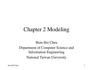
Chapter 2 Modeling of Control Systems. NUAA-Control System Engineering. How to analyze and design a control system. n. Disturbance. r. e. y. Controller. Actuator. Plant. Controlled variable. Expected value. -. Error. Sensor. u.

E N D
Chapter 2 Modeling of Control Systems NUAA-Control System Engineering
How to analyze and design a control system n Disturbance r e y Controller Actuator Plant Controlled variable Expected value - Error Sensor u • The first thing is to establish system model (mathematical model) 2
Content in Chapter 2 2-1 Introduction 2-2 Establishment of differential equation and linearization 2-3 Transfer function 2-4 Structure diagram 2-5 Signal-flow graphs 3
System model Definition: Mathematical expression of dynamic relationship between input and output of a control system. Mathematical model is foundation to analyze and design automatic control systems No mathematical modelof a physical system is exact. We generally strive to develop a model that isadequate for the problem at hand but without making the model overly complex. 5
Three models Differential equation Transfer function Frequency characteristic Study time-domain response study frequency-domain response Linear system Transfer function Differential equation Frequency characteristic Laplace transform Fourier transform 6
Modeling methods Analytic method According to Newton’s Law of Motion Law of Kirchhoff System structure and parameters the mathematical expression of system input and output can be derived. Thus, we build the mathematical model ( suitable for simple systems). 7
Modeling methods Input Black box Output System identification method Building the system model based on the system input—output signal This method is usually applied when there are little information available for the system. Neural Networks, Fuzzy Systems Black box: the system is totally unknown. Grey box: the system is partially known. 8
Why Focus on Linear Time-Invariant (LTI) System What is linear system? • -A system is called linear if the principle of superposition applies system system system Is y(t)=u(t)+2 a linear system? 9
Advantages of linear systems • The overall response of a linear system can be obtained by -- decomposing the input into a sum of elementary signals -- figuring out each response to the respective elementary signal -- adding all these responses together. Thus, we can use typical elementary signal (e.g. unit step ,unit impulse, unit ramp) to analyze system for the sake of simplicity. 10
What is time-invariant system? • A system is called time-invariant if the parameters are stationary with respect to time during system operation • Examples? 11
2.2 Establishment of differential equation and linearization 12
Differential equation Linear ordinary differential equations --- A wide range of systems in engineering are modeled mathematically by differential equations --- In general, the differential equation of an n-th order system is written Time-domain model 13
How to establish ODE of a control system --- list differential equations according to the physical rules of each component; --- obtain the differential equation sets by eliminating intermediate variables; --- get the overall input-output differential equation of control system. 14
Examples-1 RLC circuit R L C uc(t) u(t) i(t) Input Output system u(t) uc(t) Defining the input and output according to which cause-effect relationship you are interested in. 15
R L C uc(t) i(t) u(t) According to Law of Kirchhoff in electricity 16
It is re-written as in standard form • Generally,we set • the output on the left side of the equation • the input on the right side • the input is arranged from the highest order to the lowest order 17
Examples-2 Mass-spring-friction system Spring k F(t) m Displacement x(t) friction f Gravity is neglected. We are interested in the relationship between external force F(t) and mass displacement x(t) Define: input—F(t); output---x(t) 18
By eliminating intermediate variables, we obtain the overall input-output differential equation of the mass-spring-friction system. Recall the RLC circuit system These formulas are similar, that is, we canuse the same mathematical modelto describe a class of systems that arephysically absolutely different butshare the same Motion Law. 19
Examples-3 nonlinear system In reality, most systems are indeed nonlinear, e.g. then pendulum system, which is described by nonlinear differential equations. • It is difficult to analyze nonlinear systems, however, we can linearize the nonlinear system near its equilibrium point under certain conditions. 20
Linearization of nonlinear differential equations Several typical nonlinear characteristics in control system. output output input input 0 0 Saturation (Amplifier) Dead-zone (Motor) 21
Methods of linearization (1)Weak nonlinearity neglected If the nonlinearity of the component is not within its linear working region, its effect on the system is weak and can be neglected. (2)Small perturbation/error method Assumption: In the system control process, there are just small changes around the equilibrium point in the input and output of each component. This assumption is reasonable in many practical control system: in closed-loop control system, once the deviation occurs, the control mechanism will reduce or eliminate it. Consequently, all the components can work around the equilibrium point. 22
A(x0,y0) is equilibrium point. Expanding the nonlinear function y=f(x) into a Taylor series about A(x0,y0)yields Example Saturation (Amplifier) The input and output only have small variance around the equilibrium point. This is linearized model of the nonlinear component. 23
Note:this method is only suitable for systems with weak nonlinearity. Relay Saturation For systems with strong nonlinearity, we cannot use such linearization method. 24
Example-4 modeling a nonlinear system • Flash toilet Q1: inflow per unit time Q2: outflow per unit time Q10=Q20=0 Initial water level: H0 Define: Input—Q1,Output—H Problem: Derive the differential equation of water tank (the cross-sectional area of the water tank is C). 25
Solution: Outflow or inflow within dt time should be equal to the total amount of water change(Q1-Q2)dt , that is: According to ‘Torricelli Theorem’, the water yield is in direct proportion to the square root of the height of water level, thus: It is obvious that this formula is nonlinear, On the basis of the Taylor Series expansion of functions around operation points (Q10,H0 ),We have 26
Therefore, the Linearized Differential Equations of the water tank is: 27
Exercise • E1. Please build the differential equations of the following two systems. Input A Input Output x B Output 28
Solutions. (1) RC circuit (2) Mass-spring system 29
Solving Differential Equations Example Solving linear differential equations with constant coefficients: • To find the general solution (involving solving the characteristic equation) • To find a particular solution of the complete equation(involving constructing the family of a function) 31
WHY need LAPLACE transform? Time-domain ODE problems Solutions of time-domain problems s-domain algebra problems Laplace Transform (LT) Difficult Easy Solutions of algebra problems Inverse LT 32
Laplace Transform Laplace, Pierre-Simon 1749-1827 The Laplace transform of a function f(t) is defined as where is a complex variable. 33
Examples Step signal: f(t)=A • Exponential signal f(t)= 34
Properties of Laplace Transform (1) Linearity (2) Differentiation Using Integration By Parts method to prove where f(0) is the initial value of f(t). 36
(3) Integration Using Integration By Parts method to prove ) 37
(4)Final-value Theorem The final-value theorem relates the steady-state behavior of f(t) to the behavior of sF(s) in the neighborhood of s=0 (5) Initial-value Theorem 38
(6)Shifting Theorem: a. shift in time (real domain) b. shift in complex domain (7) Real convolution (Complex multiplication) Theorem 39
Inverse Laplace transform Definition:Inverse Laplace transform, denoted by is given by where C is a real constant。 Note: The inverse Laplace transform operation involving rational functions can be carried out using Laplace transform table and partial-fraction expansion. 40
Partial-Fraction Expansion method for finding Inverse Laplace Transform If F(s) is broken up into components If the inverse Laplace transforms of components are readily available, then 41
Poles and zeros • Poles • A complex number s0 is said to be a pole of a complex variable function F(s) if F(s0)=∞. • Zeros • A complex number s0 is said to be a zero of a complex variable function F(s) if F(s0)=0. Examples: zeros: 1, -2 poles: -3, -4; poles: -1+j, -1-j; zeros: -1 42
Case 1: F(s) has simple real poles Partial-Fraction Expansion Inverse LT Parameterspkgive shape and numbers ckgive magnitudes. 43
Example 1 Partial-Fraction Expansion 44
Case 2: F(s) has simple complex-conjugate poles Example 2 Laplace transform Applying initial conditions Partial-Fraction Expansion Inverse Laplace transform 45
Case 3: F(s) has multiple-order poles Simple poles Multi-order poles The coefficients corresponding to the multi-order poles are determined as 46
Example 3 Laplace transform: s= -1 is a 3-order pole Applying initial conditions: Partial-Fraction Expansion 47
Determining coefficients: Inverse Laplace transform: 48
With aid of MATLAB 1. Laplace Transform L=laplace(f) 2. Inverse Laplace Transform F=ilaplace(L) • >> syms t • >> L=laplace(t) • L= • 1/s^2 • >> L=laplace(sin(t)) • L= • 1/(s^2+1) • >> F=ilaplace(L) • F= • sin(t) 49
Transfer function LTI system Output y(t) Input u(t) Consider a linear system described by differential equation Assume all initial conditions are zero, we get the transfer function(TF) of the system as 50