Download
1 / 10
100 likes | 208 Views
Statistical Image Analysis in High-Content Microscopy Screens. Experiments by Florian Fuchs. Identify genes that are responsible for controlling cellular morphogenesis Identify genes essential for cell viability Experimental data automated fluorescent microscopy of HeLa cells; 3 channels

E N D
Statistical Image Analysis in High-Content Microscopy Screens Experiments by Florian Fuchs Identify genes that are responsible for controlling cellular morphogenesis Identify genes essential for cell viability Experimental data automated fluorescent microscopy of HeLa cells; 3 channels per well; 3 replicates; all genes Analysis preprocessing– automated image analysis of about 100000 images: reduction of information complexity of every image down to a finite set of parameters that characterize it postprocessing – statistical analysis of extracted parameters Data of the analysis image intensity and intensity distribution; image histograms; nuclei/cell counts, size and fluorescent intensity; average inter-nuclear/cellular distance, nuclei per cell, shape factors etc Tools
What the data look like... Dapi Dapi Tubulin Tubulin Phalloidin Phalloidin Dapi Dapi Tubulin Tubulin Phalloidin Phalloidin Experimental data: automated fluorescent microscopy; 3 channels per well; 3 replicates; all genes; more than 80000 images
CONTROL What we try to find... Nuclear phenotype Cytokinesis Multipolar spindles Tubulin elongation Mitotic arrest
Why using automated image analysis? Pros – amount of data is infeasible to analyse manually – automated analysis ensures objective and reproducible results! – manual analysis is done using some software anyway, why not to use it one step further – existing software (microscope experiment control software) allows only for some basic analysis steps, and on single images only – further statistical analysis is possible based on automatically generated data – automated analysis is faster and more precise in many tasks – enables creation of tools for easy browsing and reporting of images/results Contras – algorithms need to be developed and implemented! – algorithms require fine tuning of different parameters – some patterns although distinguishable to a human eye are difficult to distinguish for computers: requires a lot of fine tuning/training!
Questions and Answers Q: Why R needs image processing? A: In order to extend capabilities of R in statistical data analysis onto data of imaging Q: Any direct applications? A: Automated analysis of microscopic images from high-content screening experiments Q: Matlab has some of these functionalities already, why R? A: Open source, scalability, performance especially on large data sets Q: Is there anything already? A: Open source only Rimage, which is very limited in functionality part of Bioconductor.org development SVN branch
Manipulating Image Data im1 <- read.image(“im01.jpg”); im2 <- read.image(“im02.jpg”) # addition of two images, combining features of both in one im3 <- im1 + im2 # subtraction of images – image difference im4 <- im1 – im2 # multiplication – amplification of common features and removal of differences im5 <- im1 * im2 # scaling of data im6 <- im1 * 2 # extending contrast of dark regions im7 <- sqrt(im1) # cropping images and subscripting im8 <- im1[100:200, 80:180] im9 <- im1[100:200, ] # conditional replacement of image data – thresholding im8[im8 > 0.5] <- 1.0 # data of one image is modified based on condition from another one im1[im2 <= 0.2] <- 0.0 # conversions between colour modes and summation of RGB images rgb <- toRed(im1) + toGreen(im2); gray <- toGray(rgb) addition subtraction multiplication sqrt(im) im[..] im[im>0.4]=1
library(EBImage) w1 <- read.image(dir(pattern="w1")) w3 <- read.image(dir(pattern="w3")) w1 <- normalize(w1, independent=TRUE) w3 <- normalize(w3, independent=TRUE) w13 <- w1+w3 w13 <- normalize(w13, independent=TRUE) seg13 <- thresh(w13, 80,80,0.03, TRUE) dm13<-sqrt(distMap(seg13)) res13<-objectCount(dm13, w13, 100) seg1 <- thresh(w1, 60,60,0.03, TRUE) dm1<-sqrt(distMap(seg1)) res1<-objectCount(dm1, w13, 70) res13[[4]][1:5,] [,1] [,2] [,3] [,4] [,5] [1,] 4 328 414 1058 300.23903 [2,] 4 596 61 1176 307.50270 [3,] 4 319 3 719 182.46390 [4,] 4 625 209 993 160.84554 [5,] 4 49 0 443 80.27151
Image processing results for the whole library Dapi channel; replicate 1 > dapi$R1 ID PLATE WELL DHA_ID PROBLEM INTENSITY NOBJECTS AVDISTANCE AVSIZE 1 3 HT10-C04 A05 DHA035_A03 0 19673.72 116 40.01023 420.3621 2 5 HT10-C04 A07 DHA035_A04 0 18148.82 85 41.32718 468.5529 3 7 HT10-C04 A09 DHA035_A05 0 17935.91 83 38.55638 468.9639 4 9 HT10-C04 A11 DHA035_A06 0 17766.12 94 41.96683 469.3191 5 11 HT10-C04 A13 DHA035_A07 0 17875.37 99 39.32209 438.3333 6 13 HT10-C04 A15 DHA035_A08 0 17782.09 75 46.33427 452.7067 7 15 HT10-C04 A17 DHA035_A09 0 18852.01 111 39.06955 457.0450 8 17 HT10-C04 A19 DHA035_A10 0 18852.21 98 42.53190 469.0714 9 19 HT10-C04 A21 DHA035_A11 0 17549.30 80 41.85745 435.6375 10 21 HT10-C04 A23 DHA035_A12 8 19391.85 118 34.96427 388.2203 ... (total 18477 lines)
Image processing results for plate 26 alongside with plate reader results