Download
1 / 40
400 likes | 595 Views
2IL50 Data Structures. Spring 2014 Lecture 6: Hash Tables. Abstract Data Types. Abstract data type. Abstract Data Type ( ADT ) A set of data values and associated operations that are precisely specified independent of any particular implementation.

E N D
2IL50 Data Structures Spring 2014Lecture 6: Hash Tables
Abstract data type Abstract Data Type (ADT)A set of data values and associated operations that are precisely specified independent of any particular implementation. Dictionary, stack, queue, priority queue, set, bag …
Priority queue Max-priority queueStores a set S of elements, each with an associated key (integer value). OperationsInsert(S, x): inserts element x into S, that is, S← S⋃ {x}Maximum(S): returns the element of S with the largest keyExtract-Max(S): removes and returns the element of S with the largest keyIncrease-Key(S, x, k): give key[x] the value k condition: k is larger than the current value of key[x]
Implementing a priority queue Θ(n) Θ(1) Θ(1) Θ(n) Θ(n) Θ(1) Θ(n) Θ(n) Θ(log n) Θ(1) Θ(log n) Θ(log n)
Dictionary DictionaryStores a set S of elements, each with an associated key (integer value). OperationsSearch(S, k): return a pointer to an element x in S with key[x] = k, or NIL if such an element does not exist. Insert(S, x): inserts element x into S, that is, S← S⋃ {x} Delete(S, x): remove element x from S S: personal data • key: burger service number • name, date of birth, address, … (satellite data)
Implementing a dictionary Today hash tables Next lecture (balanced) binary search trees Θ(n) Θ(1) Θ(1) Θ(log n) Θ(n) Θ(n)
Hash tables • Hash tables generalize ordinary arrays
T 0 NIL 1 NIL 2 satellite data 3 NIL satellite data satellite data satellite data NIL satellite data 20,000,000 NIL Hash tables • S: personal data • key: burger service number (bsn) • name, date of birth, address, … (satellite data) Assume: bsn are integers in the range [0 .. 20,000,000] Direct addressinguse tableT[0 .. 20,000,000]
T 0 NIL 1 NIL 2 satellite data 3 NIL satellite data satellite data satellite data NIL satellite data M-1 NIL Direct-address tables • S: set of elements • key: unique integer from the universe U= {0,…, M-1} • satellite data • use table (array) T[0..M-1] NIL if there is no element with key i in S pointer to the satellite data if there is an element with key i in S Analysis: • Search, Insert, Delete: • Space requirements: T[i] = O(1) O(M)
Direct-address tables • S: personal data • key: burger service number (bsn) • name, date of birth, address, … (satellite data) Assume: bsn are integers with 10 digits ➨ use table T[0 .. 9,999,999,999] ?!? • uses too much memory, most entries will be NIL … • if the universe U is large, storing a table of size |U| may be impractical or impossible • often the set K of keys actually stored is small, compared to U➨ most of the space allocated for T is wasted.
T 0 NIL 1 NIL 2 3 NIL NIL 9,999,999 NIL Hash tables • S: personal data • key = bsn = integer from U = {0 .. 9,999,999,999} Idea: use a smaller table, for example, T[0 .. 9,999,999] and use only 7 last digits to determine position key = 0,130,000,003 key = 7,646,029,537 6,029,537 key = 2,740,000,003
T 0 NIL 1 NIL 2 3 NIL i NIL m-1 NIL Hash tables • S set of keys from the universe U = {0 .. M-1} • use a hash table T [0..m-1] (with m ≤ M) • use a hash function h : U → {0 … m-1} to determine the position of each key: key k hashes to slot h(k) • How do we resolve collisions?(Two or more keys hash to the same slot.) • What is a good hash function? key = k; h(k) = i
T k7 k1 k5 0 1 k2 2 k6 k4 3 4 5 k3 k9 k8 996 997 998 999 Resolving collisions: chaining Chaining: put all elements that hash to the same slot into a linked list Example (m=1000): h(k1) = h(k5) = h(k7) = 2 h(k2) = 4 h(k4) = h(k6) = 5 h(k8) = 996 h(k9) = h(k3) = 998 Pointers to the satellite data also need to be included ...
k7 k1 k5 key[x] k6 k4 k3 k9 Hashing with chaining: dictionary operations Chained-Hash-Insert(T,x)insert x at the head of the list T[h(key[x])] Time: O(1) T 0 1 x: i h(key[x]) = i k8 996 997 998 999
k6 k4 k3 k9 Hashing with chaining: dictionary operations Chained-Hash-Delete(T,x)delete x from the list T[h(key[x])] • x is a pointer to an element Time: O(1) (with doubly-linked lists) T 0 x 1 k7 k1 k5 i k8 996 997 998 999
T 0 1 k7 k1 k5 k6 k4 i k8 996 k3 k9 997 998 999 Hashing with chaining: dictionary operations Chained-Hash-Search(T, k)search for an element with key k in list T[h(k)] Time: • unsuccessful: O(1 + length of T[h(k)] ) • successful: O(1 + # elements in T[h(k)] ahead of k)
Hashing with chaining: analysis Time: • unsuccessful: O(1 + length of T[h(k)] ) • successful: O(1 + # elements in T[h(k)] ahead of k) ➨ worst case O(n) Can we say something about the average case? Simple uniform hashingany given element is equally likely to hash into any of the m slots
Hashing with chaining: analysis Simple uniform hashingany given element is equally likely to hash into any of the m slots in other words … • the hash function distributes the keys from the universe U uniformly over the m slots • the keys in S, and the keys with whom we are searching, behave as if they were randomly chosen from U ➨ we can analyze the average time it takes to search as a function of the load factorα = n/m (m: size of table, n: total number of elements stored)
Hashing with chaining: analysis TheoremIn a hash table in which collision are resolved by chaining, an unsuccessful search takes time Θ(1+α), on the average, under the assumption of simple uniform hashing. Proof (for an arbitrary key) • the key we are looking for hashes to each of the m slots with equal probability • the average search time corresponds to the average list length • average list length = total number of keys / # lists = α ■ • The Θ(1+α) bound also holds for a successful search (although there is a greater chance that the key is part of a long list). • If m = Ω(n), then a search takes Θ(1) time on average.
What is a good hash function? • as random as possibleget as close as possible to simple uniform hashing … • the hash function distributes the keys from the universe U uniformly over the m slots • the hash function has to be as independent as possible from patterns that might occur in the input • fast to compute
What is a good hash function? Example: hashing performed by a compiler for the symbol table • keys: variable names which consist of (capital and small) letters and numbers: i, i2, i3, Temp1, Temp2, … Idea: • use table of size (26+26+10)2 • hash variable name according to the first two letters:Temp1 → Te Bad idea: too many “clusters” (names that start with the same two letters)
1000001 1000001 1011010 What is a good hash function? Assume: keys are natural numbersif necessary first map the keys to natural numbers “aap” → → map bit string to natural number ➨the hash function is h: N → {0, …, m-1} • the hash function always has to depend on all digits of the input ascii representation
Common hash functions Division method: h(k) = k mod m Example: m=1024, k = 2058 ➨ h(k) = 10 • don’t use a power of 2m = 2p➨ h(k) depends only on the p least significant bits • use m = prime number, not near any power of two Multiplication method: h(k) = m (kA mod 1) • 0 < A < 1 is a constant • compute kA and extract the fractional part • multiply this value with m and then take the floor of the result • Advantage: choice of m is not so important, can choose m = power of 2
Resolving collisions more options …
T k7 k1 k5 0 1 k2 2 k6 k4 3 4 5 k3 k9 k8 996 997 998 999 Resolving collisions Resolving collisions • Chaining: put all elements that hash to the same slot into a linked list • Open addressing: • store all elements in the hash table • when a collision occurs, probe the table until a free slots is found
T 0 1 2 3 4 5 6 Hashing with open addressing Open addressing: • store all elements in the hash table • when a collision occurs, probe the table until a free slots is found Example: T[0..6] and h(k) = k mod 7 • insert 3 • insert 18 • insert 28 • insert 17 • no extra storage for pointers necessary • the hash table can “fill up” • the load factor is α is always ≤ 1 28 3 17 18 17
Hashing with open addressing • there are several variations on open addressing depending on how we search for an open slot • the hash function has two arguments: the key and the number of the current probe ➨ probe sequence ‹h(k,0), h(k, 1), … h(k, m-1)› The probe sequence has to be a permutation of ‹0, 1, … ,m-1› for every key k.
T 0 1 2 3 4 5 6 Open addressing: dictionary operations we’re actually inserting element x with key[x] = k Hash-Insert(T, k) • i = 0 • while (i < m) and (T[ h(k,i) ] ≠ NIL ) • do i = i +1 • if i < m • then T [h(k,i)] = k • else “hash table overflow” Example: Linear Probing • T[0..m-1] • h’(k) ordinary hash function • h(k,i) = (h’(k) + i) mod m • Hash-Insert(T,17) 28 17 3 18 17 17 17
T 0 1 2 3 4 5 6 Open addressing: dictionary operations Hash-Search(T,k) • i = 0 • while (i < m) and (T [ h(k,i) ] ≠ NIL) • do if T[ h(k,i) ] = k • then return “k is stored in sloth(k,i)” • elsei = i +1 • return “k is not stored in the table” Example: Linear Probing • h’(k) = k mod 7h(k,i) = (h’(k) + i) mod m • Hash-Search(T,17) 28 17 3 18 17 17 17
T 0 1 2 3 4 5 6 Open addressing: dictionary operations Hash-Search(T,k) • i= 0 • while (i < m) and (T [ h(k,i) ] ≠ NIL) • do if T[ h(k,i) ] = k • then return “k is stored in sloth(k,i)” • elsei = i +1 • return “k is not stored in the table” Example: Linear Probing • h’(k) = k mod 7h(k,i) = (h’(k) + i) mod m • Hash-Search(T,17) • Hash-Search(T,25) 28 3 18 25 17 25 25
T 0 1 2 3 4 5 6 Open addressing: dictionary operations Hash-Delete(T,k) • remove k from its slot • mark the slot with the special value DEL Example: delete 18 • Hash-Search passes over DEL values when searching • Hash-Insert treats a slot marked DEL as empty ➨ search times no longer depend on load factor ➨ use chaining when keys must be deleted 28 3 DEL 18 17
Open addressing: probe sequences • h’(k) = ordinary hash function Linear probing: h(k,i) = (h’(k) + i) mod m • h’(k1) = h’(k2) ➨ k1 and k2 have the same probe sequence • the initial probe determines the entire sequence ➨ there are only m distinct probe sequences • all keys that test the same slot follow the same sequence afterwards • Linear probing suffers from primary clustering: long runs of occupied slots build up and tend to get longer ➨ the average search time increases
Open addressing: probe sequences • h’(k) = ordinary hash function Quadratic probing: h(k,i) = (h’(k) + c1i + c2i2) mod m • h’(k1) = h’(k2) ➨ k1 and k2 have the same probe sequence • the initial probe determines the entire sequence ➨ there are only m distinct probe sequences • but keys that test the same slot do not necessarily follow the same sequence afterwards • quadratic probing suffers from secondary clustering: if two distinct keys have the same h’ value, then they have the same probe sequence Note: c1, c2, and m have to be chosen carefully, to ensure that the whole table is tested.
Open addressing: probe sequences • h’(k) = ordinary hash function Double hashing: h(k,i) = (h’(k) + i h’’(k)) mod m, h’’(k) is a second hash function • keys that test the same slot do not necessarily follow the same sequence afterwards • h’’ must be relatively prime to m to ensure that the whole table is tested. • O(m2) different probe sequences
Open addressing: analysis Uniform hashingeach key is equally likely to have any of the m! permutations of ‹0, 1, …, m-1› as its probe sequence Assume: load factor α = n/m < 1, no deletions TheoremThe average number of probes is • Θ(1/(1-α)) for an unsuccessful search • Θ((1/ α) log (1/(1-α)) ) for a successful search
n n-1 n-2 n-i+2 … m m-1 m-2 m-i+2 n ( ) i-1 ≤ = αi-1 1 m 1-α Open addressing: analysis TheoremThe average number of probes is • Θ(1/(1-α)) for an unsuccessful search • Θ((1/ α) log (1/(1-α)) ) for a successful search Proof: E [#probes] = ∑1≤ i ≤ ni ∙ Pr [# probes = i] = ∑1≤ i ≤ n Pr [# probes ≥ i] Pr [#probes ≥ i] = E [#probes] ≤∑1≤ i ≤ n αi-1 ≤ ∑0≤ i ≤ ∞ αi = ■ Check the book for details!
Implementing a dictionary • Running times are average times and assume (simple) uniform hashing and a large enough table (for example, of size 2n) Drawbacks of hash tables: operations such as finding the min or the successor of an element are inefficient. Θ(n) Θ(1) Θ(1) Θ(log n) Θ(n) Θ(n) Θ(1) Θ(1) Θ(1)