Download
1 / 74
770 likes | 929 Views
The Response of Marine Boundary Layer Clouds to Climate Change in a Hierarchy of Models. Chris Jones Department of Applied Math Advisor: Chris Bretherton Departments of Applied Math and Atmospheric Sciences. VOCALS RF05, 72W, 20S. Overview.

E N D
The Response of Marine Boundary Layer Clouds to Climate Change in a Hierarchy of Models Chris Jones Department of Applied Math Advisor: Chris Bretherton Departments of Applied Math and Atmospheric Sciences VOCALS RF05, 72W, 20S
Overview • Introduction: Marine boundary layer (MBL) clouds and climate sensitivity • Idealized local case studies in a hierarchy of models • The well-mixed MBL from observations • Comparison of model responses to changes in CO2 and temperature • Summary of proposed future work
Earth’s Radiation Budget:R = Absorbed Solar Radiation – Outgoing LongwaveRadiation Marine boundary layer clouds especially important because… They’re reflective at visible wavelengths MBL clouds (NASA)
Earth’s Radiation Budget:R = Absorbed Solar Radiation – Outgoing LongwaveRadiation CloudFraction Marine boundary layer clouds especially important because… They’re reflective at visible wavelengths They cover a lot of area Global net cloud radiative forcing ~ -20 W m-2 (Loeb et al, 2009) Compared to CO2 ~ 2 W m-2 Cloud forcing = R(clear sky) – R(all sky) (images courtesy of Chris Bretherton)
Earth’s Radiation Budget:R = Absorbed Solar Radiation – Outgoing LongwaveRadiation • Marine boundary layer clouds especially important because • They’re shiny (reflect incoming solar radiation) • They cover a lot of area • They’re hard to realistically represent in global climate models • Interplay between dynamics and physics • Nonlinear • Turbulent • Physics must be parameterized
Climate Change: Response to radiative forcingR = Absorbed Solar Radiation – Outgoing LongwaveRadiation If radiation budget is perturbed by a radiative forcing (e.g., doubling CO2),the Earth’s mean surface temperature adjusts until balance is restored: :Global mean equilibrium surface temperature change (“sensitivity to ”) Feedback parameter Cloud contribution most uncertain (next slide) W m-2K-1 (Planck) Example: If results in more low cloud, that means more reflected solar radiation, less warming ( is smaller for a given ) and thus a negative cloud feedback
Cloud feedbacks dominate climate sensitivity uncertainty in GCMs Clouds dominate overall climate feedback uncertainty Bony et al. (2006) Clouds: - Positive feedback, - Large spread between models
Cloud feedbacks dominate climate sensitivity uncertainty in GCMs Clouds dominate overall climate feedback uncertainty Bony et al. (2006) Clouds: - Positive feedback, - Large spread between models
Cloud feedbacks dominate climate sensitivity uncertainty in GCMs Clouds dominate overall climate feedback uncertainty Low clouds dominate cloud feedback uncertainty Bony et al. (2006) Soden and Vecchi (2011) Clouds: - Positive feedback, - Large spread between models
Parameterizations of Physical Processes Make Profound Impact Equilibrium response to 2xCO2 3.2K climate sensitivity 4.0 K climate sensitivity UW turbulence and shallow convection parameterizations largely responsible for increase in climate sensitivity from CAM4 to CAM5 – can our analysis help explain this? (Gettelman et al., 2011)
Objectives of This Research • Use a localized, idealized column-oriented analysis of prototypical MBL cloud regimes to identify and evaluate MBL cloud-climate radiative response mechanisms • Hierarchy of models: • Large eddy simulation (LES): high resolution cloud resolving model – closest we have to “observations” in local climate change simulations • Single-column model (SCM): ties results to GCM • Mixed-layer model (MLM): simplified model for interpretive purposes • Seek to relate SCM back to parent GCM • Scientific Relevance: Understanding mechanisms of change in GCMs is pre-requisite for constraining through observation and/or improving parameterizations. • Mathematical Relevance: Investigate impacts of various parts of model formulation (e.g., subgrid parameterizations, model resolution, applied large-scale forcings); to what extent can models be used to interpret the behavior of other models?
Case studies drawn from CGILS Intercomparison Zhang et al (2010) • S12: Shallow Stratocumulus (Sc) • Well-mixed BL • S11: Transition between Sc and shallow cumulus (Cu) • Onset of BL decoupling • Cu rising into Sc • S6: Shallow Cu
Hierarchy of models SCM (SCAM5) GCM (CAM5) SCAM5 Vertical Resolution Image courtesy of NOAA MLM LES (SAM) (S6, courtesy of Peter Blossey)
Primitive equations for liquid static energy () and total water mixing ratio () in this study Large-scale advection • Tendencies due to physical processes, e.g., • Precipitation • Radiation and clouds • Microphysics • Turbulence Subsidence Dynamics
Mixed-layer model equations • Moist static energy • Water mixing ratio • Inversion (cloud top) (Stevens, 2007)
Mixed-layer model equations (Stevens, 2007) Radiation Advective cooling/drying surface fluxes Entrainment Precipitation
How reasonable is the well-mixed assumption? Previous project studied the extent of well-mixed vs. decoupled boundary layers using aircraft data from VOCALS field experiment • Classified flight legs as well-mixed or decoupled based on gradient of moisture and temperature quantities October 2008-November 2008 (http://www.atmos.washington.edu/~robwood/VOCALS/vocals_uw.html)
Well-mixed Decoupled Cloud layer Subcloud layer • Profile-based decoupling classification: • Well-mixed if g kg-1 and K • Approximately 30% of region was well-mixed. • Well-mixed regions correspond to shallower boundary layers. • These conditions are met at S12 location. Jones et al. (2011)
Case setup and proposed sensitivity studies Simulation setup CGILS sensitivity studies Control (CTL) Mimics current climate 4xCO2 concentration (4xCO2): Captures “fast” adjustment Uniform +2K temp. increase: Captures temperature-mediated response Reduced subsidence (P2K) Subsidence as in CTL (P2K OM0) • Diurnally averaged summertime insolation • Models run to steady-state • Large-scale forcings specified from observations: • Horizontal divergence • Subsidence • Sea surface temperature • Wind profile
S12 Results: Cloud Fraction LES Results from CGILSintercomparison MLM Results
Preliminary S12 Results: Profiles Liquid static energy Moisture Cloud liquid SAM LES: MLM:
Liquid static energy Moisture Cloud liquid SAM LES: MLM: SCAM5:(L80)
Preliminary S12 Results: Summary 4xCO2 P2K P2K OM0 • All models exhibit similar steady-state mean sensitivities: • 4xCO2 has lower inversion, thinner cloud (positive cloud feedback) • P2K deepens and thickens relative to control (negative cloud feedback) • P2K OM0 thinner than P2K and slightly thinner than CTL (positive cloud feedback) • Subsidence (large scale dynamics) plays dominant role in P2K response
MLM 4xCO2 Sensitivity Mechanism: Increased down-welling LW radiation • decreased cloud top radiative cooling (~10% decrease) • Less turbulence (i.e., less entrainment) • Lower zi • Cloud thickness decreases 4xCO2 CTL 4xCO2 CTL
SCAM5 S12 Resolution Sensitivity Default CAM5 Resolution doesn’t sustain a cloud Higher resolution does Cloud fraction
Future Work • Apply MLM to interpreting other LESs involved in CGILS case study • Fully investigate SCAM5 S12 behavior • What’s driving the resolution sensitivity? • Expand analysis to other locations (MLM may not apply) • Parameter-space representation with SCAM • Use SST, Free troposphere lapse rate, CO2 and/or subsidenceas control parameters • Find a way to relate the local cloud response in SCAM to the sensitivity in its parent GCM
(MODIS satellite image) Questions?
Future Work (plenty to keep me busy) • Apply MLM to interpreting other LESs involved in CGILS case study (hypothesis: by tuning entrainment efficiency, can I reproduce their mean properties / sensitivities?) • Dig into roots of SCAM5 S12 sensitivity (interpret w/MLM when appropriate) • What’s driving the resolution sensitivity? • Expand analysis to other locations (MLM may not apply) • Parameter-space representation with SCAM, following approach of Caldwell and Bretherton (2009) MLM study • Use SST, Free troposphere lapse rate, CO2 and/or subsidenceas control parameters • Find a way to relate the local cloud response in SCAM to the sensitivity in its parent GCM
Additional Slides • CRF, adjusted CRF, etc.
SAM LES Equations • Prognostic TKE SGS model • Diagnostic cloud water, cloud ice, rain, and snow • Periodic horizontal domain, surface fluxes from Monin-Obukhov similarity theory • ISCCP cloud simulator • Parallel (MPI) Khairoutdinov and Randall (2003)
The proposal (remember the proposal? This is a presentation about the proposal …) • Use MLM to interpret output from other LESs (can “tune” parameterizations and entrainment closure as needed) • Investigate sensitivities in each model for each location • Map out primitive parameter-space representation using SCM (like CB09) • Ultimately, most concerned with SCAM, b/c it connects directly to GCM – to what extent can we use this analysis to shed light on the low cloud-climate mechanisms in CAM5?
Primitive equations for liquid static energy () and total water mixing ratio () in this study Large-scale advection • Tendencies due to physical processes, e.g., • Precipitation • Radiation and clouds • Microphysics • Surface fluxes • Turbulence Subsidence
Primitive equations • LES: • SCAM:
Mixed-layer model equations Prognostic equations: Entrainment closure: • (Moist static energy) • (total water mixing ratio) • : Inversion height • (vertical turbulent flux of x) • (radiation flux) • (precipitation) • A: entrainment efficiency
Mixed-layer model equations Prognostic equations: Mixed Layer Assumptions: • Vertically uniform profiles below inversion • Surface fluxes from bulk transfer model • Inversion flux given by • No turbulence above inversion • Precipitation parameterized following Wood et al • Radiation from RRTMG radiative transfer model • Subsidence, large scale divergence, SST, surface pressure, and free troposphere h, q specified at all times
Mixed-layer model equations: subsidence Radiative cooling Sensible heat flux Latent heat flux Precipitation Advection(cooling,drying) Entrainment warming/drying
Contributing Mechanisms for MBL Balance Subsidence Advection EPIC 2001 (Bretherton, et al.)
Mixed-layer model: • Well mixed q and h moist thermo variables => vertically uniform. • Bulk aerodynamic formulas for surface flux • Inversion fluxes based on thermo jumps subsidence Radiative cooling Sensible heat flux Latent heat flux Precipitation Advection(cooling,drying) Entrainment warming/drying
Sc (top) vs. Cu (bottom) MBL structure (Stevens et al 2007; Stevens 2006)
Relevant previous column modeling studies • Caldwell and Bretherton • Zhang and Bretherton • …
Model run specifics • Grid resolution • CESM 1.0 (CAM5): 1 deg = 0.9 deg x 1.25 deg x 30 levels • (i.e., ~100 km x 137 km x … [variable]) • Time steps (?) • Length of integration • Numerics / miscellaneous
Outline • Introduction • Climate sensitivity, feedbacks, and cloud radiative forcing • Why are low clouds important (to climate system, climate sensitivity)? • What has been done, and where does this study fit in? • Feedback flow chart (?) • Proposal for this study: Localized case studies using a hierarchy of models • CGILS cases • Primitive equations • An assortment of models • GCM (global models, under-resolved,…) • SCM (single column of the GCM) • LES (high-resolution column model – resolve largest, most energetic eddies, models subgrid) • MLM (idealized reduced order model that uses • Decoupling work pepper VOCALS throughout • MLM comparison with LES for S12 (and maybe SCAM?) • Proposed dissertation topic
Outline • Introduction • What is climate sensitivity and why do we care? • Why are low clouds important (to climate system, climate sensitivity)? • What has been done, and where does this study fit in? • Feedback flow chart (?) • Proposal for this study • CGILS cases • Primitive equations • An assortment of models • GCM (global models, under-resolved,…) • SCM (single column of the GCM) • LES (high-resolution column model – resolve largest, most energetic eddies, models subgrid) • MLM (idealized reduced order model that uses • Decoupling work pepper VOCALS throughout • MLM comparison with LES for S12 (and maybe SCAM?) • Proposed dissertation topic
Our approach: • Consensus that we need better understanding of the processes underlying low-cloud response to climate change (i.e., GCM intercomparison studies demonstrate clearly the global average low cloud response is a big uncertainty, but individual models differ in parameterizations of cloud processes, and climate-change output diverges widely between models) • Use IDEALIZED LOCAL CASE STUDIES (drawn from CGILS intercomparison) to investigate cloud sensitivity in a hierarchy of models (LES, SCM, and MLM) to climate-change inspired tests, with the goals of: • Understanding mechanisms behind cloud sensitivity (i.e., do LES and SCM agree? Can this behavior be constrained by observations? Is improved parameterization, informed by LES necessary?) • Connecting these back to the GCM behavior of a given model.
Proposal: use a hierarchy of models to investigate low cloud response to climate perturbations • Local analysis: • Focus on 3 regions used in CGILS intercomparison study representing 3 low cloud regimes with idealized large scale forcings • Use 3 types of column models to investigate cloud sensitivity to a variety of perturbations: • Ultimate goal: Connect these back to GCM
Profiles Well-mixed Decoupled Cloud layer Surface layer drizzle (actual cloud base – “well-mixed” cloud base) Subcloud legs