Download
1 / 59
600 likes | 723 Views
Learn how to price options using different models, hedge a stock portfolio, and evaluate employee stock options. Explore the Black-Scholes-Merton model and implied volatility. Calculate option prices and values effectively.

E N D
16 Option Valuation
Learning Objectives Make sure the price is right by making sure that you have a good understanding of: 1. How to price options using the one-period and two-period binomial models. 2. How to price options using the Black-Scholes model. 3. How to hedge a stock portfolio using options. 4. The workings of employee stock options.
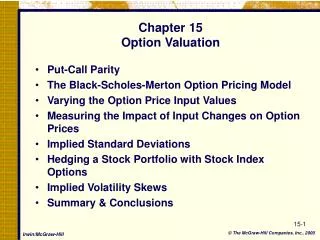
Option Valuation • Our goal in this chapter is to discuss how to calculate stock option prices. • We will discuss many details of the very famous Black-Scholes-Merton option pricing model. • We will discuss "implied volatility," which is the market’s forward-looking uncertainty gauge.
Just What is an Option Worth? • In truth, this is a very difficult question to answer. • At expiration, an option is worth its intrinsic value. • Before expiration, put-call parity allows us to price options. But, • To calculate the price of a call, we need to know the put price. • To calculate the price of a put, we need to know the call price. • So, we want to know the value of a call option: • Before expiration, and • Without knowing the price of the put
A Simple Model to Value Options Before Expiration, I. • Suppose we want to know the price of a call option with • One year to maturity. • A $110 exercise price. • The current stock price is $108. • The one-year risk-free rate, r, is 10 percent. • We know (somehow) that the stock price will be $130 or $115 in one year. • The stock price in one year is still uncertain. • We know that the stock price is going to be $130 or $115 (but no other values). • We do not know the probabilities of these two values. • Therefore, we know the call option value at expiration will be: • $130 – $110 = $20 OR • $115 - $110 = $5 • This call option is certain to finish in the money. • A similar put option is certain to finish out of the money.
A Simple Model to Value Options Before Expiration, II. • If you know the price of a similar put, you can use put-call parity to price a call option before it expires. • The chosen pair of stock prices guarantees that the call option finishes in the money. • Suppose, however, we want to allow the call option to expire in the money OR out of the money. • How do we proceed in this case? Well, we need a different option pricing model.
The One-Period Binomial Option Pricing Model—The Assumptions • Suppose the stock price today is S, and the stock pays no dividends. • We assume that the stock price in one period is either S ×u or S ×d, where: • u (for “up” factor) is bigger than 1 • and d (for “down” factor) is less than 1 • Suppose the stock price today is $100, and u = 1.1 and d = .95. • The stock price in one period will either be • $100 × 1.1 = $110 or • $100 × .95 = $95. • What is the call price today, if: • K = 100 • R = 3%
The One-Period Binomial Option Pricing Model—The Setup • Consider the following portfolio: • Buy a fractional share of the underlying asset--this fraction is represented by the Greek letter, D (Delta) • Sell one call option • Finance the difference by borrowing the amount: DS – C • Key Question: What is the value of this portfolio, today and at option expiration?
Cu and Cd: The intrinsic value of the call if the stock price increases to S×u or decreases to S×d. Portfolio Value Today Portfolio Value At Expiration The Value of this Portfolio(long D Shares and short one call) is: Important: DS is NOT the change in S. Rather, it is a dollar amount, DS. DS×u - Cu DS - C DS×d - Cd
To Calculate Today’s Call Price, C: • A Brilliant Insight: There is one combination of a fractional share and one call that makes this portfolio risk-less. • That is, the portfolio will have the same value when the underlying asset increases as it does when the underlying asset decreases in value. • The portfolio is riskless if: DSu – Cu = DSd – Cd • We know all values in this equation today, except D. • S = $100; Su = $110; Sd = $95 • Cu = MAX(Su – K, 0) = MAX($110 – 100,0) = $10. • Cd = MAX(Sd – K, 0) = MAX($95 – 100,0) = $0.
Therefore, Our First Step is to Calculate D To make the portfolio riskless: DSu – Cu = DSd – Cd DSu – DSd = Cu – Cd D(Su – Sd) = Cu – Cd, Therefore, we can calculate D: D = (Cu – Cd) / (Su – Sd) D = (10 – 0) / 110 – 95 D = 10 / 15 D = 2 / 3.
Sidebar: What is D? • D, delta, is the riskless hedge ratio. • D, delta, is the fractional share amount needed to hedge one call. • Therefore, the number of calls to hedge one share is 1/D.
The One-Period Binomial Option Pricing Model—The Formula • A riskless portfolio today should be worth (DS – C)(1+r) in one period. • So, (DS – C)(1+r) = DSu – Cu (which equals DSd – Cd because we chose the “correct” D). • Solving the equation above for C:
Now We Can Calculate the Call Price, C. What is the price of a similar put? Using Put-Call Parity: Why can we use Put-Call Parity?
The Two-Period Binomial Option Pricing Model • Suppose there are two periods to expiration instead of one. What do we do in this case? • It turns out that we repeat much of the process we used in the one-period binomial option pricing model. • This method can be used to price: • European call options. • European put options. • American calls and puts (with a modification to allow for early exercise). • An exotic array of options (with the appropriate modifications).
The Method We can find binomial option prices for two (or more) periods by using the following five steps: • Build a price “tree” for stock prices through time. • Use the intrinsic value formula to calculate the possible option values at expiration. • Calculate the fractional share needed to form each riskless portfolio at the next-to-last date. • Calculate all possible option prices at the next-to-last date. • Repeat this process by working back to today.
The Binomial Option Pricing Model with Many Periods • When there are more than two periods, nothing really changes—we just keep working on back to today.
What Happens When the Number of Periods Gets Really, Really Big? • We can always use a computer to handle this situation. • However, for European options on non-dividend paying stocks, the binomial method converges to the Black-Scholes option pricing formula. • To calculate the prices of many other types of options, however, we still need to use a computer (and methods similar in spirit to the binomial method).
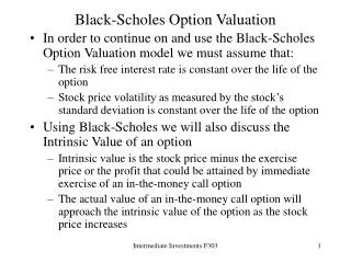
The Black-Scholes Option Pricing Model • The Black-Scholes option pricing model allows us to calculate the price of a call option before maturity (and, no put price is needed). • Dates from the early 1970s • Created by Professors Fischer Black and Myron Scholes • Made option pricing much easier—The CBOE was launched soon after the Black-Scholes model appeared. • The Black-Scholes option pricing model calculates the price of European options on non-dividend paying stocks.
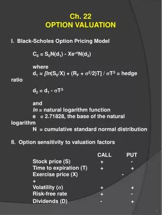
The Black-Scholes Option Pricing Model • The Black-Scholes option pricing model says the value of a stock option is determined by five factors: • S, the current price of the underlying stock. • K, the strike price specified in the option contract. • r, the risk-free interest rate over the life of the option contract. • T, the time remaining until the option contract expires. • , (sigma) which is the price volatility of the underlying stock.
The Black-Scholes Option Pricing Formula • The price of a call option on a single share of common stock is: C = SN(d1) – Ke–rTN(d2) • The price of a put option on a single share of common stock is: P = Ke–rTN(–d2) – SN(–d1) d1 and d2 are calculated using these two formulas:
Formula Details • In the Black-Scholes formula, three common functions are used to price call and put option prices: • e-rt, or exp(-rt), is the natural exponent of the value of –rt (in common terms, it is a discount factor) • ln(S/K) is the natural log of the "moneyness" term, S/K. • N(d1) and N(d2) denotes the standard normal probability for the values of d1 and d2. • In addition, the formula makes use of the fact that: N(-d1) = 1 - N(d1)
Example: Computing Pricesfor Call and Put Options • Suppose you are given the following inputs: S = $50 K = $45 T = 3 months (or 0.25 years) s= 25% (stock volatility) r = 6% • What is the price of a call option and a put option, using the Black-Scholes option pricing formula?
We Begin by Calculating d1 and d2 Now, we must compute N(d1) and N(d2). That is, the standard normal probabilities.
Using the =NORMSDIST(x) Function in Excel • If we use =NORMSDIST(1.02538), we obtain 0.84741. • If we use =NORMSDIST(0.90038), we obtain 0.81604. • Let’s make use of the fact N(-d1) = 1 - N(d1). N(-1.02538) = 1 – N(1.02538) = 1 – 0.84741 = 0.15259. N(-0.90038) = 1 – N(0.90038) = 1 – 0.81604 = 0.18396. • We now have all the information needed to price the call and the put.
The Call Price and the Put Price: • Call Price = SN(d1) – Ke–rTN(d2) = $50 x0.84741 – 45 x e-(0.06)(0.25) x 0.81604 = 50 x 0.84741 – 45 x 0.98511 x 0.81604 = $6.195. • Put Price = Ke–rTN(–d2) – SN(–d1) = $45 x e-(0.06)(0.25) x0.19479 – 50 x 0.15259 = 45 x 0.98511 x 0.18396 – 50 x 0.15259 = $0.525.
We can Verify Our Results Using Put-Call Parity Note: The options must have European-style exercise. Verified.
Using a Web-based Option Calculator • www.numa.com.
Varying the Option Price Input Values • An important goal of this chapter is to show how an option price changes when only one of the five inputs changes. • The table below summarizes these effects.
Varying the Underlying Stock Price • Changes in the stock price has a big effect on option prices.
Calculating the Impact of Stock Price Changes on Option Prices • Option traders must know how changes in input prices affect the value of the options that are in their portfolio. • An important effect on option prices is how changes in the stock price affects option prices. • The street name for this effect is “Delta.” • The other inputs also affect the option price, but we will concentrate on Delta.
Calculating Delta • Deltameasures the dollarimpact of a change in the underlying stock price on the value of a stock option. Call option delta = N(d1) > 0 Put option delta = –N(–d1) < 0 • A $1 change in the stock price causes an option price to change by approximately delta dollars.
The "Delta" Prediction: • The call delta value of 0.8474 predicts that if the stock price decreases by $1, the call option price will decrease by $0.85. • If the stock price is $49, the call option value is $5.368—an actual decrease of about $0.83. • How well does Delta predict if the stock price changes by $0.25? • The put delta value of -0.1526 predicts that if the stock price decreases by $1, the put option price will increase by $0.15. • If the stock price is $49, the put option value is $0.698—an actual increase of about $0.17. • How well does Delta predict if the stock price changes by $0.25?
Hedging with Stock Options • You own 1,000 shares of XYZ stock AND you want protection from a price decline. • Let’s use stock and option information from before—in particular, the “delta prediction” to help us hedge. • Here you want changes in the value of your XYZ shares to be offset by the value of your options position. That is:
Hedging Using Call Options—The Prediction • Using a Delta of 0.8474 and a stock price decline of $1: You should write 12 call options with a $45 strike to hedge your stock.
Hedging Using Call Options—The Results • XYZ Shares fall by $1—so, you lose $1,000. • What about the value of your option position? • At the new XYZ stock price of $49, each call option is now worth $5.37—a decrease of $.83 for each call ($83 per contract). • Because you wrote 12 call option contracts at $6.20 (rounded), your call option gain was $996 = ($6.20 - $5.37) ×12 ×100. • Your call option gain nearly offsets your loss of $1,000. • Why is it not exact? • Call Delta falls when the stock price falls. • Therefore, you did not sell quite enough call options.
Hedging Using Put Options—The Prediction • Using a Delta of -0.1526 and a stock price decline of $1: You should buy 66 put options with a strike of $45 to hedge your stock.
Hedging Using Put Options—The Results • XYZ Shares fall by $1—so, you lose $1,000. • What about the value of your option position? • At the new XYZ stock price of $49, each put option is now worth $.70—an increase of $.17 for each put ($17 per contract). • Because you bought 62 put option contracts at $.53 (rounded), your put option gain was $1,122 = ($.70 - $.53) × 66 ×100. • Your put option gain more than offsets your loss of $1,000. • Why is it not exact? • Put Delta also falls (gets more negative) when the stock price falls. • Therefore, you bought too many put options—this error is more severe the lower the value of the put delta. • To get closer: Use a put with a strike closer to at-the-money.
Hedging a Portfolio with Index Options • Many institutional money managers use stock index options to hedge the equity portfolios they manage. • To form an effective hedge, the number of option contracts needed can be calculated with this formula: • Note that regular rebalancing is needed to maintain an effective hedge over time. Why? Well, over time: • Underlying Value Changes • Option Delta Changes • Portfolio Value Changes • Portfolio Beta Changes
Example: Calculating the Number of Option Contracts Needed to Hedge an Equity Portfolio • Your $10,000,000 portfolio has a beta of 1.00. • You decide to hedge the value of this portfolio with the sale of call options. • The call options have a delta of 0.579 • The value of the index is 1508. So, you sell 115 call options.
Implied Standard Deviations • Of the five input factors for the Black-Scholes option pricing model, only the stock price volatility is not directly observable. • A stock price volatility estimated from an option price is called an implied standard deviation (ISD) or implied volatility (IVOL). • Calculating an implied volatility requires: • All other input factors, and • Either a call or put option price
CBOE Implied Volatilities for Stock Indexes • The CBOE publishes data for three implied volatility indexes: • S&P 500 Index Option Volatility, ticker symbol VIX • S&P 100 Index Option Volatility, ticker symbol VXO • NASDAQ 100 Index Option Volatility, ticker symbol VXN • The VIX, VXO, and VXN indexes are estimates of expected market volatility. • The VIX was once known as the “investor fear gauge.” • This name stems from the belief that the VIX reflects investors’ collective prediction of near-term market volatility, or risk. • Generally, the VIX increases during times of high financial stress and decreases during times of low financial stress. • Some investors use the VIX as a buy-sell indicator. • The market saying is: “When the VIX is high, it’s time to buy; when the VIX is low, it’s time to go!”
Employee Stock Options, ESOs • Essentially, an employee stock option is a calloption that a firm grants (i.e., gives) to employees. • ESOs allow employees to buy shares of stock in the company. • Giving stock options to employees is a widespread practice. • Because you might soon be an ESO holder, an understanding of ESOs is important.
Features of ESOs • ESOs have features that ordinary call options do not. • The details vary by firm, but: • The life of the ESO is generally 10 years. • ESOs cannot be sold. • ESOs have a “vesting” period of about 3 years. • Employees cannot exercise their ESOs until they have worked for the company for this vesting period. • If an employee leaves the company before the ESOs are “vested," the employees lose the ESOs. • If an employee stays for the vesting period, the ESOs can be exercised any time over the remaining life of the ESO.
Why are ESOs Granted? • Owners of a corporation (i.e., the stockholders) have a basic problem. How do they get their employees to make decisions that help the stock price increase? • ESOs are a powerful motivator, because payoffs to options can be large. • High stock prices: ESO holders gain and shareholders gain. • ESOs have no upfront costs to the company. • ESOs can be viewed as a substitute for ordinary wages. • Therefore, ESOs are helpful in recruiting employees.