Download
1 / 34
350 likes | 429 Views
Dynamic Behavior of Closed-Loop Control Systems. 4-20 mA. Chapter 11. Chapter 11.

E N D
Dynamic Behavior of Closed-Loop Control Systems 4-20 mA Chapter 11
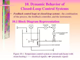
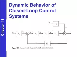
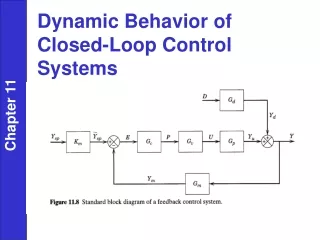
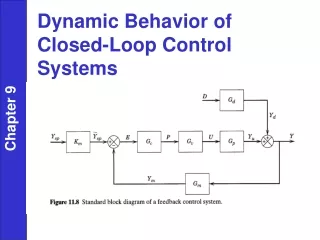
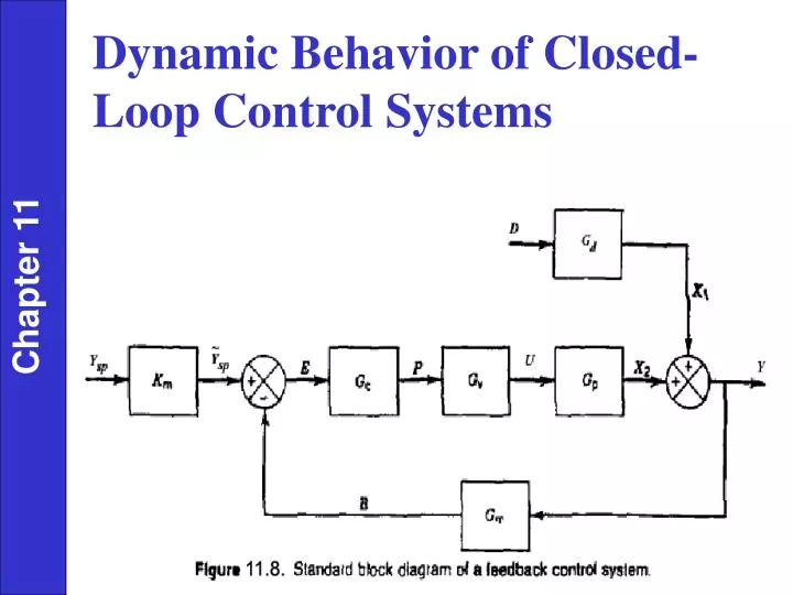
Next, we develop a transfer function for each of the five elements in the feedback control loop. For the sake of simplicity, flow rate w1 is assumed to be constant, and the system is initially operating at the nominal steady rate. Process In section 4.3 the approximate dynamic model of a stirred-tank blending system was developed: Chapter 11 where
or after taking Laplace transforms, The symbol denotes the internal set-point composition expressed as an equivalent electrical current signal. This signal is used internally by the controller. is related to the actual composition set point by the composition sensor-transmitter gain Km: Chapter 11 Thus
Current-to-Pressure (I/P) Transducer Because transducers are usually designed to have linear characteristics and negligible (fast) dynamics, we assume that the transducer transfer function merely consists of a steady-state gain KIP: Chapter 11 Control Valve As discussed in Section 9.2, control valves are usually designed so that the flow rate through the valve is a nearly linear function of the signal to the valve actuator. Therefore, a first-order transfer function usually provides an adequate model for operation of an installed valve in the vicinity of a nominal steady state. Thus, we assume that the control valve can be modeled as
Composition Sensor-Transmitter (Analyzer) We assume that the dynamic behavior of the composition sensor-transmitter can be approximated by a first-order transfer function: Controller Suppose that an electronic proportional plus integral controller is used. From Chapter 8, the controller transfer function is Chapter 11 where and E(s) are the Laplace transforms of the controller output and the error signal e(t). Note that and e are electrical signals that have units of mA, while Kc is dimensionless. The error signal is expressed as
1. Summer 2. Comparator Chapter 11 3. Block • Blocks in Series are equivalent to...
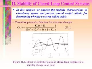
Closed-Loop Transfer Function for Set-Point Change (Servo Problem)
Closed-Loop Transfer Function for Load Change (Regulator Problem)
O I Chapter 11
EXAMPLE 1: P.I. control of liquid level Block Diagram: Chapter 11
Assumptions 1. q1, varies with time; q2 is constant. 2. Constant density and x-sectional area of tank, A. 3. (for uncontrolled process) 4. The transmitter and control valve have negligible dynamics (compared with dynamics of tank). 5. Ideal PI controller is used (direct-acting). Chapter 11 For these assumptions, the transfer functions are:
The closed-loop transfer function is: (11-68) Substitute, (2) Chapter 11 Simplify, (3) Characteristic Equation: (4) Recall the standard 2nd Order Transfer Function: (5)
To place Eqn. (4) in the same form as the denominator of the T.F. in Eqn. (5), divide by Kc, KV, KM : Comparing coefficients (5) and (6) gives: Chapter 11 Substitute, For 0 < < 1 , closed-loop response is oscillatory. Thus decreased degree of oscillation by increasing Kc or I (for constant Kv, KM, and A). • unusual property of PI control of integrating system • better to use P only