Download

1 / 37
370 likes | 441 Views
A multiline LTE inversion using PCA. Marian Martínez González. E. In astrophysics we can not directly measure the physical properties of the objects, we do always retrieve them. We are always dealing with inversion problems.

E N D
A multiline LTE inversion using PCA Marian Martínez González
E In astrophysics we can not directly measure the physical properties of the objects, we do always retrieve them. We are always dealing with inversion problems. We model the physical mechanisms that takeplace in theline formation. We model the Sun as a set of parameters contained in what we call amodel atmosphere.
E In astrophysics we can not directly measure the physical properties of the objects, we do always retrieve them. We are always dealing with inversion problems. We model the physical mechanisms that takeplace in theline formation. STOKES VECTOR We model the Sun as a set of parameters contained in what we call amodel atmosphere.
E In astrophysics we can not directly measure the physical properties of the objects, we do always retrieve them. We are always dealing with inversion problems. We model the physical mechanisms that takeplace in theline formation. STOKES VECTOR We model the Sun as a set of parameters contained in what we call amodel atmosphere.
Model atmosphere: - Temperature (pressure, density) profile along the optical depth. - Bulk velocity profile. - Magnetic field vector variation with depth. - Microturbulent velocity profile. - Macroturbulent velocity. Let’s define the vector containing all the variables: = [T,v,vmic,vmac,B,...] Mechanism of line formation Local Thermodynamic Equilibrium. Population of the atomic levels Saha-Boltzmann Energy transport The radiative transport is the most efficient. Radiative transfer equation. S = f()
Model atmosphere: - Temperature (pressure, density) profile along the optical depth. - Bulk velocity profile. - Magnetic field vector variation with depth. - Microturbulent velocity profile. - Macroturbulent velocity. Let’s define the vector containing all the variables: = [T,v,vmic,vmac,B,...] Mechanism of line formation Local Thermodynamic Equilibrium. Population of the atomic levels Saha. Energy transport The radiative transport is the most efficient. Radiative transfer equation. OUR PROBLEM OF INVERSION IS: S = f() = finv(S)
= finv(S) sol The information of the atmospheric parameters is encoded in the Stokes profiles in a non-linear way. Iterative methods (find the maximal of a given merit function) Sobs ini ± Forward modelling ini NO Steor Merit function Converged? Sobs YES
The noise in the observational profiles induce that: • Several maximals with similar amplitudes are possible in the merit • function. • This introduces degeneracies in the parameters. • We are not able to detect these errors!
The noise in the observational profiles induce that: • Several maximals with similar amplitudes are possible in the merit • function. • This introduces degeneracies in the parameters. • We are not able to detect these errors! • BAYESIAN INVERSION OF STOKES PROFILES • Asensio Ramos et al. 2007, A&A, in press • - Samples the Likelihood but is very slow. • PCA INVERSION BASED ON THE MILNE-EDDINGTON APPROX. • López Ariste, A. • - Finds the global minima of a 2 but the number of parameters increases in a multiline • analysis.
A single model atmosphere is needed to reproduce as spectral lines • as wanted. • Does not get stuck in local minima. • We can give statistically significative errors. • It is faster than the SIR code. • It can be a very good initialitation for the SIR code. But, at its present state... • It is limited to a given inversion scheme (namely, the number of • nodes) • - The data base seems to be not complete enough. We propose a PCA inversion code based on the SIR performance
A single model atmosphere is needed to reproduce as spectral lines • as wanted. • Does not get stuck in local minima. • We can give statistically significative errors. • It is faster than the SIR code. • It can be a very good initialitation for the SIR code. But, at its present state... • It is limited to a given inversion scheme (namely, the number of • nodes) • - The data base seems to be not complete enough. We propose a PCA inversion code based on the SIR performance More work has to be done... and I hope to receive some suggestions!!
PCA inversion algorithm DATA BASE Steor↔ Principal Components Pi i=0,..,N Each observed profile can be represented in the base of eigenvectors: Sobs=iPi We compute the projection of each one of the observed profiles in the eigenvectors: iobs= Sobs · Pi ; i=0,..,n<<N PCA allows compression!! SVDC Sobs iteor = Steor· Pi Compute the 2 search in Find the minimum of the 2
PCA inversion algorithm DATA BASE Steor↔ Principal Components Pi i=0,..,N Each observed profile can be represented in the base of eigenvectors: Sobs=iPi We compute the projection of each one of the observed profiles in the eigenvectors: iobs= Sobs · Pi ; i=0,..,n<<N PCA allows compression!! SVDC Sobs How do we construct a COMPLETE data base??? iteor = Steor· Pi This is the very key point Compute the 2 search in Find the minimum of the 2
PCA inversion algorithm DATA BASE Steor↔ Principal Components Pi i=0,..,N Each observed profile can be represented in the base of eigenvectors: Sobs=iPi We compute the projection of each one of the observed profiles in the eigenvectors: iobs= Sobs · Pi ; i=0,..,n<<N PCA allows compression!! SVDC Sobs How do we construct a COMPLETE data base??? iteor = Steor· Pi This is the very key point How do we compute the errors of the retrieved parameters?? Are they coupled to the non-completeness of the data base ?? Compute the 2 search in Find the minimum of the 2
SIR Montecarlo generation of the profiles of the data base i=0,.... ?? from a random uniform distribution Is there any other similar profile in the data base ??? i Siteor 2(Siteor, Sjteor) < ; j ≠ i i=i+1 YES NO Save irej i=i+1 Add it to the data base
SIR Montecarlo generation of the profiles of the data base i=0,.... ?? from a random uniform distribution Is there any other similar profile in the data base ??? i Siteor 2(Siteor, Sjteor) < ; j ≠ i Which are these parameters?? i=i+1 YES NO Save irej i=i+1 Add it to the data base
Modelling the solar atmosphere 13 independent variables • - A field free atmosphere (occupying a fraction 1-f): • Temperature: 2 nodes linear perturbations. • Bulk velocity: constant with height. • Microturbulent velocity: constant with height. • - A magnetic atmosphere (f): • Temperature: 2 nodes. • Bulk velocity: constant. • Microturbulent velocity: constant. • Magnetic field strength: constant. • Inclination of the field vector with respect to the LOS: constant. • Azimuth of the field vector: constant. • - A single macroturbulent velocity has been used to convolve the • Stokes vector.
Synthesis of spectral lines The idea is to perform the synthesis as many lines as are considered of interest to study the solar atmosphere. In order to make the numerical tests we use the following ones: Fe I lines at 630 nm Fe I lines at 1.56 m Spectral synthesis We use the SIR code. Ruiz Cobo, B. et al. 1992, ApJ, 398, 375 Reference model atmosphere HSRA (semiempirical) Gingerich, O. et al. 1971, SoPh, 18, 347
SIR Montecarlo generation of the profiles of the data base i=0,.... ?? from a random uniform distribution Is there any other similar profile in the data base ??? i Siteor 2(Siteor, Sjteor) < ; j ≠ i i=i+1 YES NO Save irej i=i+1 Add it to the data base
SIR Montecarlo generation of the profiles of the data base i=0,.... ?? from a random uniform distribution Is there any other similar profile in the data base ??? i Siteor 2(Siteor, Sjteor) < ; j ≠ i We use the noise level as the reference i=i+1 YES NO Save irej i=i+1 Add it to the data base
SIR Montecarlo generation of the profiles of the data base i=0,.... ?? from a random uniform distribution Is there any other similar profile in the data base ??? i Siteor 2(Siteor, Sjteor) < ; j ≠ i i=i+1 YES NO Save irej i=i+1 Add it to the data base
SIR Montecarlo generation of the profiles of the data base i=0,.... ?? from a random uniform distribution How many do we need in order the base to be “complete” ?? Is there any other similar profile in the data base ??? i Siteor 2(Siteor, Sjteor) < ; j ≠ i i=i+1 YES NO Save irej i=i+1 Add it to the data base
SIR Montecarlo generation of the profiles of the data base i=0,.... ?? from a random uniform distribution How many do we need in order the base to be “complete” ?? The data base will never be complete.. We have created a data base with ~65000 Stokes vectors. Is there any other similar profile in the data base ??? i Siteor 2(Siteor, Sjteor) < ; j ≠ i i=i+1 YES NO Save irej i=i+1 Add it to the data base
Degeneracies in the parameters Studying the data base: Degeneracies in the parameters = 10-3 Ic 1.56 m ~ 25 % of the proposed profiles have been rejected. The noise has made the B, f, parameters not to be. For magnetic flux densities lower than ~50 Mx/cm2 the product of the three magnitudes is the only observable.
Degeneracies in the parameters Studying the data base: Degeneracies in the parameters = 10-4 Ic 1.56 m ~ 11 % of the proposed profiles have been rejected. The noise has made the B, f, parameters not to be. For magnetic flux densities lower than ~8 Mx/cm2 the product of the three magnitudes is the only observable.
Degeneracies in the parameters Studying the data base: Degeneracies in the parameters = 10-4 Ic 630 m +1.56 m ~ 0.7 % of the proposed profiles have been rejected!! The noise has made the B, f, parameters not to be. For magnetic flux densities lower than ~4 Mx/cm2 the product of the three magnitudes is the only observable.
Testing the inversions = 10-3 Ic 1.56 m
Testing the inversions = 10-3 Ic 1.56 m
Testing the inversions = 10-3 Ic 1.56 m
Testing the inversions = 10-3 Ic 1.56 m
Testing the inversions = 10-3 Ic 1.56 m
Testing the inversions = 10-3 Ic 1.56 m
Testing the inversions = 10-3 Ic 1.56 m The errors are high but close to the supposed error of the data base
Testing the inversions = 10-4 Ic 630 nm + 1.56 m
Testing the inversions = 10-4 Ic 630 nm + 1.56 m Apart from some nice fits, it is impossible to retrieve any of the parameters with a data base of 65000 profiles!!
- The inversions should work for two spectral lines with ~105 profiles in the data base for a polarimetric accuracy of 10-3-10-4 Ic. - The inversion of a lot of spectral lines proves to be very complicated using PCA inversion techniques. - IT IS MANDATORY TO REDUCE THE NUMBER OF PARAMETERS. - The model atmospheres would be represented by some other parameters that are not physical quantities (we would not depend on the distribution of nodes) but that reduce the dimensionality of the problem and correctly describes it.