Download
1 / 30
300 likes | 487 Views
G53BIO - Bioinformatics Phylogenetic Trees. Dr. Jaume Bacardit http://www.cs.nott.ac.uk/~jqb/G53BIO. Examples from D.A.Krane & M.L. Raymer ’ s “ Fundamental Concepts of Bioinformatics ” and from D.W. Mount ’ s “ Bioinformatics: Sequence and Genome Analysis ”. Outline.

E N D
G53BIO - BioinformaticsPhylogenetic Trees Dr. Jaume Bacardit http://www.cs.nott.ac.uk/~jqb/G53BIO Examples from D.A.Krane & M.L. Raymer’s “Fundamental Concepts of Bioinformatics” and from D.W. Mount’s “Bioinformatics: Sequence and Genome Analysis”
Outline • Introduction and motivation • Types of trees • Algorithms to construct trees • UPGMA • Fitch-Margoliash • Neighbour-Joining • Sources of information
Aims • Phylogeny has the goals of working out the relationships among species, populations, individuals or genes (taxa in a general sense) • The results of phylogenetic analysis are usually presented as a collection of nodes and branches. That is, a tree • In such tree, taxa that are closely related in an evolutionary sense appear close to each other, and taxa that are distantly related are in different (far) branches of the trees • Phylogenetic trees are also important for multiple sequence alignment • Various… • Types of tree exists • Sources of information to generate the trees • Ways to generate the trees
Trees are usually bifurcating but it is also possible to have multifurcating trees • Interpretation: • At some point in the past an ancestral population gave rise to more than 2 lineages or • Insufficient/erroneous data impedes the discrimination of the true nature of the tree thus coalescing various branches into one multifurcating one. • Not only the topology of the trees convey information, also the relative sizes of the branches: • Scaled trees: branch length are proportional to the differences between pairs of neighbouring nodes. • Additive trees: these are scaled trees in which the physical length of the branches connecting two nodes is an accurate representation of their accumulated differences • Unscaled trees: only convey kinship information
Phylogenetic Trees can be: • Rooted: A single node is designated as root and it represents a common ancestor with a unique path leading from it through evolutionary time to any other node • Unrooted tree: specifies only the nodes interrelations but says nothing about the direction in which evolution occurred. Roots can be artificially assigned to unrooted trees by means of an outgroup. An outgroup is a species that have unambiguously separated early from the other species being considered Example: comparing Humas and Gorilas, Baboons could be used as outgroups and the root would be placed somewhere along the branch conecting Baboons to the common ancestors for Humans and Gorilas.
Rooted trees Unrooted trees
Number of Rooted VS Unrooted Trees NR = (2n -3)!/ 2^(n-2) * (n – 2)! NU = (2n – 5)!/ 2^(n-3) * (n – 3)! But only one of these represents the true turn of events! Most phylogenetic trees generated with molecular data are thus referred to as inferred trees.
Unweighted pair group method with arithmetic meant (UPGMA) • The oldest tree reconstructions method (1960) • Requires a distance matrix, e.g.:
E.G. dAB represents the distance between species A & B, while dAC is the distance between taxa A & C, etc UPGMA: • Cluster the two species with the smallest distance putting then into a single group. Assume that in the example dAB is the smallest, hence a new group (AB) is created. • Recalculate the distance matrix with the new group (AB) against C and D: • d(AB)C = 0.5 * (dAC+dBC) • d(AB)D = 0.5 * (dAD+dBD) • With the new distance matrix repeat 1 until all species have been grouped.
Fitch-Margoliash Algorithm Main idea: • Sequences are first combined into groups of three and used to calculated branches’ length. • Sequences are added progresively • Branch lengths are assumed to be additive • Then join all sequences in pair, assess their inferred distances and calculate a percentage squared error • Repeat with different initialisation until finding a good (small error) tree
Fitch-Margoliash Algorithm • From the distance matrix find the closest pair, e.g., A & B • Treat the rest of the sequences as a single composite sequence. Calculate the average distance from A to all of the other sequences and B to all of the other sequences • Use these values to calculate the distances a and b between A and the joining common node to B and the same for B. • Take A and B as a single composite sequence AB, calculate the average distances between AB and each of the other sequences, and make a new distance table from these values. • Indentify the next pair of most closely related sequences and proceed as in step 1 to calculate the next set of branch length. • When necessary substract extended branch lengths to calculate lengths of intermediate branches. • Repeat the entire procedure starting with all possible pairs of sequences A and B, A and C, A and D, etc • Calculate the predicted distances between each pair of sequences for each tree to find the tree that best fits the original data
D a D and E are the closest sequences c A-C b E a = 4 b = 6 c = 29 Now let’s recompute the complate distance matrix
C a b is not just for that segment, it represents the complete distance from the connecting node to the leaves C and DE are the closet sequences c A-B b DE a = 9 b = 10 c = 31 Now let’s recompute the complate distance matrix C 9 31 A-B 5 4 D 6 E
B Now we are in thee trivial case of 3 sequences b b is not just for that segment, it represents the complete distance from the connecting node to the leaves c A a CDE a = 29.5 b = 10 c = 12 A C 9 10 This time we got the perfect tree. However, this is not always the case. The algorithm should be repeated with different initial pairings (who are A and B) and then compare the difference between the actual and predicted distnaces (from summing the length of the branches) 20 5 4 12 B D 6 E
Neighbour Joining Algorithm • Similar to Fitch-Margoliash except that sequences are paired based on the effect of the pairing on the sum of the branch lengths of the tree. • The general Neighbour Joining algorithm can be downloaded from ftp.virginia.edu/pub/fasta/GNJ
The Algorithm 1. The distances between pair of objects are used to calculate the sum of the branch length for a tree that has no preferred pairing of sequences.
Decompose the star-like tree by combining pairs of sequences. Using the same example as before this gives:
Each possible sequence pair is chosen and the sum of the branch lengths of the corresponding tree is calculated. For the example: S_AB=67.7, S_BC=81, S_CD=76, S_DE=70 plus six other possibilities. • Choose the one with the lowest sum, in this case S_AB. • Once the choice is made calculate the brachn lengths a,b and the average distance from AB to CDE using FM method: • a = [d_AB + (d_AC+d_AD+d_AE)/3 – (d_BC+d_BD+d_DE)/3]/2 = (22 + 39.7 -41.7)/2 = 10 • b = [ d_AB +(d_BC+d_BD+d_BE)/3 – (d_AC+d_AD+d_AE)/3]/2 = (22 + 41.7 +39.7)/2 = 12
6. Like in Fitch-Margoliash method: A new distance table with A and B forming a single composite sequence is produced and the algorithm is iterated from the beginning to find the next sequence pair and the next branch lengths.
Sources of information • So far, all methods shown computed the distance matrix between species from a set of aligned sequences (DNA or Protein) • There are many more sources of information • Complete genomes • Restriction sites • Non-coding DNA regions
Tree of life constructed from all species for which their complete genome has been sequenced
Summary • There are several methods to compute phylogenetic trees, and sources of information • Need to be familiar with several of them to appreciate their differences • There are various guiding mechanisms to choose how to build the trees based on likelihood functions and information theory • Get familiar with Phylip package as it is a standard one • Other programs exist