Download

1 / 65
650 likes | 683 Views
Building Phylogenetic Trees. Yaw-Ling Lin ( 林耀鈴 ) Dept Computer Sci and Info Management Providence University, Taiwan E-mail: yllin@pu.edu.tw WWW: http://www.cs.pu.edu.tw/~yawlin. branch. internal node. leaf. Phylogenetic Tree. Topology: bifurcating Leaves - 1 … N

E N D
Building Phylogenetic Trees Yaw-Ling Lin (林耀鈴) Dept Computer Sci and Info Management Providence University, Taiwan E-mail: yllin@pu.edu.tw WWW: http://www.cs.pu.edu.tw/~yawlin
branch internal node leaf Phylogenetic Tree • Topology: bifurcating • Leaves - 1…N • Internal nodes N+1…2N-2
Counting Trees A B A C C D B C D A E B C A D E B F (2N - 5)!! = # unrooted trees for N taxa (2N- 3)!! = # rooted trees for N taxa
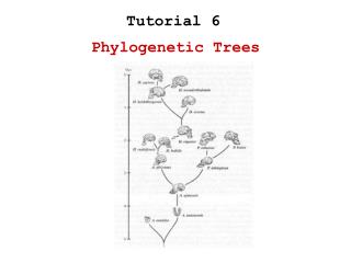
B C Root D A A C B D Rooted tree Note that in this rooted tree, taxon A is no more closely related to taxon B than it is to C or D. Root Rrooting the tree: To root a tree mentally, imagine that the tree is made of string. Grab the string at the root and tug on it until the ends of the string (the taxa) fall opposite the root: Unrooted tree
UPGMA -- Unweighted Pair Group Method with Arithmetic mean A A B B dAB / 2 C d(AB)C / 2 A B B dAB C dAC dBC simplest method - uses sequential clustering algorithm (assumption of rate constancy among lineages - often violated) step 1 step 2 (AB) C d(AB)C Distance matrix Tree d(AB)C = (dAC + dAB) / 2
d a e b c UPGMA Step 1combine B and C
d a 2 2 e b c UPGMA step 2combine BC and D (10+12)/2 (4+6)/2
2 .5 .5 d a 2 2 e b c UPGMA step 3combine A and E
2 .5 3.5 3.5 .5 d a 2 2 e b c UPGMA step 4combine AE and BCD
2 .5 3.5 2.5 3.5 3.5 .5 d a 2 2 e b c UPGMA Result
2 .5 3.5 2.5 3.5 3.5 .5 d a 2 2 e b c UPGMA Result
Neighbor Joining • Very popular method • Does not make molecular clock assumption : modified distance matrix constructed to adjust for differences in evolution rate of each taxon • Produces unrooted tree • Assumes additivity: distance between pairs of leaves = sum of lengths of edges connecting them • Like UPGMA, constructs tree by sequentially joining subtrees
Naïve NJ by Additivity? • O(n2) (i,j) pairs • O(n2) (k,l) pairs • (k,l) “rejects” (i,j) whenever additivity fails • O(n4) to pick an (i,j) neighbor pair! • So totally O(n5) time suffices
j i j i k m Neighbor-Joining: Algorithm
Neighbor-Joining: Complexity • The method performs a search using time O(n2) and using time O(n2) to update distance matrix. • Giving a total time complexity of O(n3),and a space complexity of O(n2).
Reasoning the NJ Method • How did the ideas of Si,j and Ri comes from ? • How correct is the algorithm? • Heuristic or exact solution?
The “1-star” Sum of the Branch Lengths • D and L as the distance between OTUs and the branch length between nodes • Each branch is counted N-1 times when all distances are added
3 1 2 4 Lemma
3 1 2 4 Proof
Proof of the Theorem: by contradiction r k i s Type1: A = -2Dux-2Duv Type2: B =-4Dvx+2Duv For the sum in formula b to be nonnegative, Type2 should be more than Type1. w B x x u v x A j l Suppose that i and j are not neighbors. Let k and l be any pair of neighbors, so that i, j, k, and l are distinct and are represented in the tree .Consider the sum in formula (b), which is nonnegative. If m is fifth OUT, then it joins the tree at point x along one of the indicated arcs. Say that m is of type 1 if it joins the path from I to j at any node different from u and that m is of type 2 if it joins the path from i to j at node u.
Proof of the theorem (Cont.) If m is of type 1,then the corresponding summand in formula (b) is -2Dux-2Duv. If m is of type 2, then the corresponding summand in formula (b) is -4Dvx+2Duv. For the sum in formula (b) to be nonnegative, there must be at least as many terms corresponding to OTUs m of type 2 as there are terms corresponding top OTUs m of type 1. It follows that there are more OTUs that join the path from i to j at u than there are OTUs that join that path at all other nodes combined. Because neither i nor j has a neighbor, there must be a pair r,s of neighbors that argument applied to w that is different from u, By the above argument applied to w, there are more OTUs that join the path from i to j at w than there are OTUs that join that path at all other nodes combined. The conclusions about u and w contradict each other, and the theorem follows.
Speeding up Neighbor-Joining Tree Construction • In this paper, the authors present several heuristics for speeding up the NJ method. • The heuristics attempt to reduce the search time by using a quad-tree. • The worst case time complexity remains O(n3) and the space complexity after adding the quad-tree is still O(n2). • The authors have implemented a tool, QuickJoin.
Previous Work • The neighbor-joining method is introduced by Saitou and Nei. • The algorithm was later amended by Studier and Keppler with a running time O(n3). • BIONJ -- Gascuel et al. produce a O(n3) implementation of a variant of the NJ algorithm that produce more accurate trees in many cases. • QuickTree -- Durbin et al. produce an code optimized implementation of the NJ algorithm.
+/- of distance methods • Advantages: • easy to perform • quick calculation • fit for sequences having high similarity scores • Disadvantages: • the sequences are not considered as such (loss of information) • all sites are generally equally treated (do not take into account differences of substitution rates ) • not applicable to distantly divergent sequences.
Maximum Parsimony Method Site OTU 1 2 3 4 5 6 7 8 9 10 1 2 3 4 T C A G A T C T A G T T A G A A C T A G T T C G A T C G A G T T C T A A G G A C principle - search for tree that requires the smallest number of character state changes between the OTUs informative sites - those that favor some trees over others operationally - at least two different kinds of residues at the site, each of which is found in at least two of the OUT sequences
Evaluating Parsimony Scores • How do we compute the Parsimony score for a given tree? • Traditional Parsimony • Each base change has a cost of 1 • Weighted Parsimony • Each change is weighted by the score c(a,b)
a g a Traditional Parsimony a {a} • Solved independently for each position • Linear time solution a {a,g}
k j i Evaluating Weighted Parsimony Dynamic programming on the tree Initialization: • For each leaf i set S(i,a) = 0 if i is labeled by a, otherwise S(i,a) = Iteration: • if k is node with children i and j, then S(k,a) = minb(S(i,b)+c(a,b)) + minb(S(j,b)+c(a,b)) Termination: • cost of tree is minaS(r,a) where r is the root
Cost of Evaluating Parsimony • Score is evaluated on each position independetly. Scores are then summed over all positions. • If there are n nodes, m characters, and k possible values for each character, then complexity is O(nmk) • By keeping traceback information, we can reconstruct most parsimonious values at each ancestor node
Inferring trees – Maximum Likelihood method • Maximum likelihood supposes a model of evolution along tree branches. • Strategy: Find parameters (tree, branch lengths, substitution rate) that maximizes the likelihood assigned to the data. • Note: Model of evolution does not include indels! • In Phylip package: program PROTML