Download
1 / 35
350 likes | 395 Views
Scheduling Criteria. CPU utilization – keep the CPU as busy as possible (from 0% to 100%) Throughput – # of processes that complete their execution per time unit Turnaround time – amount of time to execute a particular

E N D
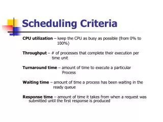
Scheduling Criteria CPU utilization – keep the CPU as busy as possible (from 0% to 100%) Throughput – # of processes that complete their execution per time unit Turnaround time – amount of time to execute a particular Process Waiting time – amount of time a process has been waiting in the ready queue Response time – amount of time it takes from when a request was submitted until the first response is produced
Optimization Criteria • Max CPU utilization • Max throughput • Min turnaround time • Min waiting time • Min Response time
Scheduling Algorithems • First Come First Serve Scheduling • Shortest Job First Scheduling • Priority Scheduling • Round-Robin Scheduling • Multilevel Queue Scheduling • Multilevel Feedback-Queue Scheduling
First Come First Serve Scheduling (FCFS) ProcessBurst time P1 24 P2 3 P2 3
First Come First Serve Scheduling • The average of waiting time in this policy is usually quite long • Waiting time for P1=0; P2=24; P3=27 • Average waiting time= (0+24+27)/3=17
First Come First Serve Scheduling • Suppose we change the order of arriving job P2, P3, P1
First Come First Serve Scheduling • Consider if we have a CPU-bound process and many I/O-bound processes • There is a convoy effect as all the other processes waiting for one of the big process to get off the CPU • FCFS scheduling algorithm is non-preemptive
Short job first scheduling (SJF) • This algorithm associates with each process the length of the processes’ next CPU burst • If there is a tie, FCFS is used • In other words, this algorithm can be also regard as shortest-next-cpu-burst algorithm
Short job first scheduling • SJF is optimal – gives minimum average waiting time for a given set of processes
Example ProcessesBurst time P1 6 P2 8 P3 7 P4 3 FCFS average waiting time: (0+6+14+21)/4=10.25 SJF average waiting time: (3+16+9+0)/4=7
Short job first scheduling Two schemes: Non-preemptive – once CPU given to the process it cannot be preempted until completes its CPU burst Preemptive – if a new process arrives with CPU burst length less than remaining time of current executing process, preempt. This scheme is know as the Shortest-Remaining-Time-First (SRTF)
Priority Scheduling A priority number (integer) is associated with each process The CPU is allocated to the process with the highest priority (smallest integer ≡ highest priority) • Preemptive • Non-preemptive SJF is a special priority scheduling where priority is the predicted next CPU burst time, so that it can decide the priority
Priority Scheduling ProcessesBurst timePriorityArrival time P1 10 3 P2 1 1 P3 2 4 P4 1 5 P5 5 2 The average waiting time=(6+0+16+18+1)/5=8.2
Priority Scheduling ProcessesBurst timePriorityArrival time P1 10 3 0.0 P2 1 1 1.0 P3 2 4 2.0 P4 1 5 3.0 P5 5 2 4.0 Gantt chart for both preemptive and non-preemptive, also waiting time
Priority Scheduling Problem : Starvation – low priority processes may never execute Solution : Aging – as time progresses increase the priority of the process
Round-Robin Scheduling • The Round-Robin is designed especially for time sharing systems. • It is similar FCFS but add preemption concept • A small unit of time, called time quantum, is defined
Round-Robin Scheduling • Each process gets a small unit of CPU time (time quantum), usually 10-100 milliseconds. After this time has elapsed, the process is preempted and added to the end of the ready queue.
Round-Robin Scheduling • If there are n processes in the ready queue and the time quantum is q, then each process gets 1/n of the CPU time in chunks of at most q time units at once. No process waits more than (n-1)q time units.
Round-Robin Scheduling Performance • q large => FIFO • q small => q must be large with respect to context switch, otherwise overhead is too high • Typically, higher average turnaround than SJF, but better response
Multilevel Queue Ready queue is partitioned into separate queues: • foreground (interactive) • background (batch) Each queue has its own scheduling algorithm foreground – RR background – FCFS
Multilevel Queue example • Foreground P1 53 (RR interval:20) P2 17 P3 42 • Background P4 30 (FCFS) P5 20
Multilevel Queue Scheduling must be done between the queues • Fixed priority scheduling; (i.e., serve all from foreground then from background). Possibility of starvation. • Time slice – each queue gets a certain amount of CPU time which it can schedule amongst its processes; i.e., 80% to foreground in RR
Multilevel Feedback Queue Three queues: • Q0 – RR with time quantum 8 milliseconds • Q1 – RR time quantum 16 milliseconds • Q2 – FCFS Scheduling A new job enters queue Q0 which is served FCFS. When it gains CPU, job receives 8 milliseconds. If it does not finish in 8 milliseconds, job is moved to queue Q1. At Q1 job is again served FCFS and receives 16 additional milliseconds. If it still does not complete, it is preempted and moved to queue Q2.
Multilevel Feedback Queue • P1 40 • P2 35 • P3 15
5.4 Multiple-Processor Scheduling • We concentrate on systems in which the processors are identical (homogeneous) • Asymmetric multiprocessing (by one master) is simple because only one processor access the system data structures. • Symmetric multiprocessing, each processor is self-scheduling. Each processor may have their own ready queue.
Load balancing • On symmetric multiprocessing systems, it is important to keep the workload balanced among all processors to fully utilized the benefits of having more than one CPU • There are two general approached to load balancing: Push Migration and Pull Migration
Symmetric Multithreading • An alternative strategy for symmetric multithreading is to provide multiple logical processors (rather than physical) • It’s called hyperthreading technology on Intel processors
Symmetric Multithreading • The idea behind it is to create multiple logical processors on the same physical processor (sounds like two threads) • But it is not software provide the feature, but hardware • Each logical processor has its own architecture state, each logical processor is responsible for its own interrupt handling.