Download
1 / 18
180 likes | 334 Views
Observing Convection in Stellar Atmospheres. John Landstreet London, Canada. Introduction. Convection reaches photosphere in most stars of T e < 10 4 K, perhaps also in hotter stars Directly visible in Sun as granulation

E N D
Observing Convection in Stellar Atmospheres John Landstreet London, Canada IAU Symposium 239
Introduction • Convection reaches photosphere in most stars of Te < 104 K, perhaps also in hotter stars • Directly visible in Sun as granulation • Detected in stars as microturbulence, macroturbulence, bisector curvature, etc • Comparison of convection models with observed spectra provides interpretation of observations and tests of models IAU Symposium 239
Solar granulation • Appearance of sun with good seeing reveals granulation • Sequences of images suggest coherent overturning flow • Granulation ~ visible convection cells • => Study convection observationally IAU Symposium 239
Indirect detection of velocity fields • Granulation not directly visible on (unresolved) stellar surfaces • But velocity fields in photosphere affect spectral line profiles & energy distribution, so we may still study convection observationally • Simplest example of velocity field: stellar rotation • Small for “cool” stars, large for “hot” stars IAU Symposium 239
Microturbulence • Abundance analysis allows indirect detection of small-scale velocity field (excess line broadening over thermal), required to fit weak and strong lines • Microturbulence parameter x characterizes velocity • Required for most stars with Te < 10000 K, corresponds to convective instability • => Microturbulence ~ convection, at least in cooler stars • Detectable even in broad-line stars – much data IAU Symposium 239
Convection effects on line profiles • In Sun-like flow, expect rising and descending gas to have different velocities along line of sight • Different areal coverage (filling factors) and brightness lead to different contributions to total flux • Result: spectral lines are shifted and asymmetric • Importance of these effects depends on where in atmosphere the lines are formed – weak lines will be different from strong lines IAU Symposium 239
Macroturbulence • Most main sequence stellar line profiles can be roughly modelled with Voigt profile + rotation • Line profiles of giants & supergiants more “pointed”, with broad shallow wings • Successful model: radial-tangential macroturbulence. On half of surface, lines have Gaussian spread radially, on other half lines have Gaussian spread tangentially. • One parameter: macroturbulence zRT (velocity) IAU Symposium 239
Macroturbulence - 2 • If zRT > 0, we conclude that large-scale velocity field exists within stellar atmosphere • => Velocity field may be studied by modelling spectral line shapes • Values vary systematically over cooler part of HR diagram • Large values of macroturbulence found among (low v sin i) main sequence A stars near Te ~ 8000K • Macroturbulence drops to zero above A0V IAU Symposium 239
Macroturbulence - 3 • Among hotter stars (Te > 10000) situation is quite confusing • For hot main sequence and giant stars, microturbulence takes various values between 0 and several km/s, but not systematically – are these values really > 0 (e.g. Lyubimkov et al 2004)? • B and A supergiants have microturbulence of several km/s, and macroturbulence of 15 – 20 km/s (e.g. Przybilla et al 2006)! • Is supergiant macroturbulence due to winds, non-radial pulsations, convection, or…? IAU Symposium 239
Radial velocities • In convecting stars (x > 0), radial velocity of lines observed to vary with line strength • Reflects typical velocity (average over flows) at depth where line is formed • Difficult to study: requires very accurate lab wavelengths, sharp lines • Not yet studied over full HR diagram • Examples: Sun, Procyon (Allende Prieto et al 2002) IAU Symposium 239
Bisector curvature (asymmetry) • Line asymmetry (bisector curvature) reveals asymmetric flows • Should provide a direct means to observe convective velocity field in photosphere • Cool stars bisectors resemble solar bisector, but with considerable variations • Gray & Nagel (1989) found bisectors reversed in hotter stars: a “granulation boundary” • Two “different” types of convection?? IAU Symposium 239
Bisector curvature (asymmetry) - 2 • On MS, reversed bisectors also found among A stars (Te <10500 K) • Late B stars show no bisector curvature, and have x < 1 km/s • Bisector curvature not studied for hotter stars, mainly because so few have v sin i < 5 km/s IAU Symposium 239
Multi-parameter models of flow • Modelling of cool stars by Dravins (1990) with four-component flow (2 hot upflows, 1 neutral, 1 cool downflow) reproduces line profiles reasonably and supports general picture of flow behaviour • Frutiger et al (2000, 2005) have used multi-parameter models to derive temperature and velocity structure of simple geometrical flow models for Sun, a Cen A & B • Useful for searches of parameter space IAU Symposium 239
3D hydrodynamic models • Physically realistic modelling requires 3D hydrodynamic models (e.g. Nordlund & Dravins) but such models are very costly • 3D models of low-metal stars with convection reveal that temperature stratification is changed significantly, perhaps also changing derived Li abundance (Asplund & Garcia Perez 2001) IAU Symposium 239
3D models - 2 • Detailed model of Procyon allows comparison of micro- macro-turbulence fits to fits of 3D line profiles (Allende Prieto et al 2002) • Without free model parameters (except fundamental parameters of star), 3D model lines provide excellent fit to observations IAU Symposium 239
3D models - 3 • CO5BOLD code used to compute coarse model of entire M2 I star; find giant convection cells as suggested by images (Freytag et al 2002) • Same code computed convective models of A star, but found no reversed bisectors (Steffen et al 2005) • Limitation of 3D codes – if one disagrees with observation, testing changes is very costly IAU Symposium 239
MLT and other convection models • MLT, FST and non-local convection models provide alternative description • Comparisons of predictions of such models with Balmer lines, uvby colours of star (Smalley & Kupka 1997; Gardiner et al 1999) show that observational tests of models are possible • Kupka & Montgomery (2002) seem to predict correct sense of A star bisectors from non-local convection model IAU Symposium 239
Conclusions • Stellar atmospheric velocity fields clearly detectable in spectrum: microturbulence, macroturbulence, bisector curvature, energy distribution,…. • Behaviour over HR diagram quite varied; largest velocities in supergiants • Modelling making progress at connecting convection theory with observations IAU Symposium 239