Download
1 / 21
210 likes | 353 Views
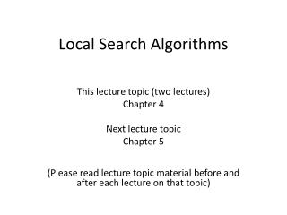
Local Search Algorithms. This lecture topic Chapter 4.1-4.2 Next lecture topic Chapter 5 (Please read lecture topic material before and after each lecture on that topic). Outline. Hill-climbing search Gradient Descent in continuous spaces Simulated annealing search Tabu search

E N D
Local Search Algorithms This lecture topic Chapter 4.1-4.2 Next lecture topic Chapter 5 (Please read lecture topic material before and after each lecture on that topic)
Outline • Hill-climbing search • Gradient Descent in continuous spaces • Simulated annealing search • Tabu search • Local beam search • Genetic algorithms • Linear Programming
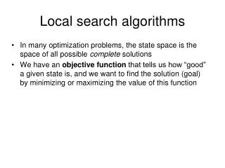
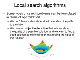
Local search algorithms • In many optimization problems, the path to the goal is irrelevant; the goal state itself is the solution • State space = set of "complete" configurations • Find configuration satisfying constraints, e.g., n-queens • In such cases, we can use local search algorithms • keep a single "current" state, try to improve it. • Very memory efficient (only remember current state)
Example: n-queens • Put n queens on an n × n board with no two queens on the same row, column, or diagonal Note that a state cannot be an incomplete configuration with m<n queens
Hill-climbing search • "Like climbing Everest in thick fog with amnesia"
Hill-climbing search: 8-queens problem • h = number of pairs of queens that are attacking each other, either directly or indirectly (h = 17 for the above state) Each number indicates h if we move a queen in its corresponding column
Hill-climbing search: 8-queens problem • A local minimum with h = 1 (what can you do to get out of this local minima?)
Hill-climbing Difficulties • Problem: depending on initial state, can get stuck in local maxima
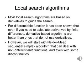
Gradient Descent • Assume we have some cost-function: and we want minimize over continuous variables X1,X2,..,Xn 1. Compute the gradient : 2.Take a small step downhill in the direction of the gradient: 3. Check if 4. If true then accept move, if not reject. 5. Repeat.
Line Search • In GD you need to choose a step-size. • Line search picks a direction, v, (say the gradient direction) and searches along that direction for the optimal step: • Repeated doubling can be used to effectively search for the optimal step: • There are many methods to pick search direction v. Very good method is “conjugate gradients”.
Newton’s Method Basins of attraction for x5 − 1 = 0; darker means more iterations to converge. • Want to find the roots of f(x). • To do that, we compute the tangent at Xn and compute where it crosses the x-axis. • Optimization: find roots of • Does not always converge & sometimes unstable. • If it converges, it converges very fast
Simulated annealing search • Idea: escape local maxima by allowing some "bad" moves but gradually decrease their frequency. • This is like smoothing the cost landscape.
Simulated annealing search • Idea: escape local maxima by allowing some "bad" moves but gradually decrease their frequency
Properties of simulated annealing search • One can prove: If T decreases slowly enough, then simulated annealing search will find a global optimum with probability approaching 1 (however, this may take VERY long) • However, in any finite search space RANDOM GUESSING also will find a global optimum with probability approaching 1 . • Widely used in VLSI layout, airline scheduling, etc.
Tabu Search • Almost any simple local search method, but with a memory. • Recently visited states are added to a tabu-list and are temporarily excluded from being visited again. • This way, the solver moves away from already explored regions and (in principle) avoids getting stuck in local minima. • Tabu search can be added to most other local search methods to obtain a variant method that avoids recently visited states. • Tabu-list is usually implemented as a hash table for rapid access. Can also add a LIFO queue to keep track of oldest node. • Unit time cost per step for tabu test and tabu-list maintenance.
Local beam search • Keep track of k states rather than just one. • Start with k randomly generated states. • At each iteration, all the successors of all k states are generated. • If any one is a goal state, stop; else select the k best successors from the complete list and repeat. • Concentrates search effort in areas believed to be fruitful. • May lose diversity as search progresses, resulting in wasted effort.
Genetic algorithms • A successor state is generated by combining two parent states • Start with k randomly generated states (population) • A state is represented as a string over a finite alphabet (often a string of 0s and 1s) • Evaluation function (fitness function). Higher values for better states. • Produce the next generation of states by selection, crossover, and mutation
Fitness function: number of non-attacking pairs of queens (min = 0, max = 8 × 7/2 = 28) • P(child) = 24/(24+23+20+11) = 31% • P(child) = 23/(24+23+20+11) = 29% etc fitness: #non-attacking queens probability of being regenerated in next generation
Linear Programming Problems of the sort: • Very efficient “off-the-shelves” solvers are available for LRs. • They can solve large problems with thousands of variables.
Linear Programming Constraints • Maximize: z = c1 x1 + c2 x2 +…+ cn xn • Primary constraints: x10, x20, …, xn0 • Additional constraints: • ai1 x1 + ai2 x2 + … + ain xn ai, (ai 0) • aj1 x1 + aj2 x2 + … + ajn xn aj 0 • bk1 x1 + bk2 x2 + … + bkn xn= bk 0
Summary • Local search maintains a complete solution • Seeks to find a consistent solution (also complete) • Path search maintains a consistent solution • Seeks to find a complete solution (also consistent) • Goal of both: complete and consistent solution • Strategy: maintain one condition, seek other • Local search often works well on large problems • Abandons optimality • Always has some answer available (best found so far)