Download
1 / 70
700 likes | 796 Views
Iterative Row Sampling. Richard Peng. CMU MIT. Joint work with Mu Li (CMU) and Gary Miller (CMU). Outline. Matrix Sketches Existence Samples better samples Iterative algorithms. Data. n-by-d matrix A , m entries Columns: data Rows: attributes. A. Goal:

E N D
Iterative Row Sampling Richard Peng CMU MIT Joint work with Mu Li (CMU) and Gary Miller (CMU)
Outline • Matrix Sketches • Existence • Samples better samples • Iterative algorithms
Data • n-by-d matrix A, m entries • Columns: data • Rows: attributes A Goal: • Classification/ clustering • Identify patterns • Interpret new data
Linear Model • Can add/scale data points • x1: coefficients,combo: Ax x3A:,3 x2A:,2 Ax x1A:,1
Problem Interpret new data point b as combination of known ones Ax ?
Regression • Express as combination of current examples • Regression:minx ║Ax–b║ p • p=2: least squares • p=1: compressive sensing • ║x║2: Euclidean norm of x • ║x║1: sum of absolute values
Variants of Compressive Sensing • minx ║Ax-b║1 +║x║1 • minx║Ax-b║2 +║x║1 • minx ║x║1s.t.Ax=b • minx ║Ax║1s.t.Bx= y • minx║Ax-b║1 + ║Bx- y║1 All similar to minx║Ax-b║1
Simplified • minx║Ax–b║p= minx║[A,b] [x; -1]║p • Regression equivalent to min║Ax║p with one entry of x fixed x A b -1
‘Big’ Data Points • Each data point has many attributes • #rows (n) >> #columns (d) • Examples: • Genetic data • Time series (videos) • Reverse (d>>n) also common: images + SIFT A
Faster? A’ A Smaller, equivalent A’ Matrix sketch
Row Sampling • Pick some rows of A to be A’ • How to pick? Random A’ A
Shorter Equivalent • Find shorter A’ that preserves answer • |Ax|p≈1+ε|A’x|p for all x • Run algorithm on A’, same answer good for A A’ Simplified error notation ≈: a≈kb if there exists k1, k2s.t. k2/k1 ≤ k and k1a ≤ b ≤ k2 b
Outline • Matrix Sketches • How? Existence • Samples better samples • Iterative algorithms
Sketches Exist |Ax|p≈|A’x|p for all x • Linear sketches: A’=SA • [Drinealset al. `12]:Row sampling: one non-zero in each row of S • [Clarkson-Woodruff `12]:S = countSketch, one non-zero per column. A’
Sketches Exist Hidden: runtime costs, ε-2dependency
WHY is ≈d possible? |Ax|p≈|A’x|p for all x • ║Ax║22 = xTATAx • ATA: d-by-dmatrix • Any factorization (e.g. QR) of ATA suffices as A’
ATA A:,j1 A:,j2 • Covariance matrix • Dot product of all pairs of columns (data) • Covariance:cov(j1,j2) = ΣiAi,j1TAi,j2
Use of Covariance Matrix • Clustering: l2 distances of all pairs given by C • Kernel methods: all pair dot products suffice for many models. C=ATA C
Other Use of Covariance • Covariance of attributes used to tune parameters • Images + SIFT: many data points, few attributes. • http://www.image-net.org/: 14,197,122 images 1000 SIFT features C
How Expensive is this? • d2 dots of length n vectors • Total: O(nd2) • Faster: O(ndω-1) • Expensive: nd2 > nd > m C A
Equivalent View Of Sketches • Approximate covariance matrix: C’=(A’)TA’ • ║Ax║2≈║A’x║2 is the same as C ≈ C’ A’ C’
Application of Sketches • A’: n’ rows • d2 dots of length n’ vectors • Total cost: O(n’dω-1) A’ C’ A
Sketches in Input Sparsity Time • Need: cost of computing C’ < cost of computing C = ATA • 2 goals: • n’ small • A’ found efficiently A’ C’ A
Outline • Matrix Sketches • How? Existence • Samples better samples • Iterative algorithms
Previous Approaches A miracle happens • Go go poly(d) rows directly • Projection to obtain key info, or the sketch itself A’ A poly(d) m
Our Main Approach • Utilize the robustness of sketches, covariance matrices, and sampling • Iteratively reduce errors and sizes A” A’ A
Composing Sketches O(n’dlogd +dω) O(m) Total cost: O(m + n’dlogd + dω) = O(m + dω) A” A’ A n’ = d1+α n rows dlogd rows
Accumulation of Errors ║Ax║2 ≈kk’║A’x║2 ║A”x║2≈k’║A’x║2 ║Ax║2≈k║A”x║2 A” A’ A n’ = d1+α n rows dlogd rows
Accmulation of Errors • Final error: product of both errors • Dependency of error in cost: usually ε-2 or more for 1± ε error • [Avron & Toledo `11]: only final step needs to be accurate • Idea: compute sketches indirectly ║Ax║ 2≈kk’║A’x║2
Row Sampling • Pick some rows of A to be A’ • How to pick? Random A’ A
Are All Rows Equal? column with one entry one non-zero row A A |A[1;0;…;0]|p≠ 0
Row Sampling • τ’ : weights on rows distribution • Pick a number of rows independently from this distribution, rescale to form A’ A’ A
Matrix Chernoff Bounds • Sufficient property of τ’ • τ: statistical leverage scores • If τ' ≥ τ,║τ'║1logd (scaled) rows suffices for A’≈ A τ' A
Statistical Leverage Scores • Studied in stats since 70s • Importance of rows • leverage score of row i, Ai: • τi= Ai(ATA)-1AiT • Key fact: ║τ║1 = rank ≤ d • ║τ'║1logd = dlogd rows τ A
Computing Leverage scores • τi= Ai(ATA)-1AiT • = AiC-1AiT • ATA: covariance matrix, C • Given C-1, can compute each τiin O(d2) time • Total cost: O(nd2+dω)
Computing Leverage scores • τi= AiC-1AiT • =║AiC-1/2║22 • 2-norm of a vector, AiC-1/2 • rows in isotropic positions • Decorrelates columns
Aside: What is Leverage? Ai AiC-1/2 • Geometric view: • Rows define ‘energy’ directions. • Normalize so total energy is uniform • τi: norm of row i after normalizing
Aside: What is Leverage? • How to interpret statistical leverage scores? • Statistics ([Hoaglin-Welsh `78], [Chatterjee-Hadi `86]): • Influence on data set • Likelihood of outlier • Uniqueness of Row τ A
Aside: What is Leverage? • High Leverage Score: • Key attribute? • Outlier (measuring error)?
Aside: What is Leverage? • My current view (motivated by graph sparsification): • Sampling probabilities • Use them to find sketches τ A
Computing Leverage scores τi= ║AiC-1/2║22 • Only need τ' ≥ τ • Can use approximations after scaling them up • Error leads to larger ║τ'║1
Dimensionality Reduction x Gx ║x║22 ≈jl║Gx║22 • Johnson Lindenstrauss Transform • G: d-by-O(1/α) Gaussian • Errorjl = dα
Estimating Leverage scores τi=║AiC-1/2║22 ≈jl║AiC-1/2G║22 • G: d-by-O(1/α) Gaussian • C1/2G: d-by-O(1/α) • Cost: O(α ∙ nnz(Ai))total: O(α ∙ m + α ∙ d2logd)
Estimating Leverage scores τi=║AiC-1/2║ 22 ≈║AiC’-1/2║ 22 • C ≈k C’ gives ║C-1/2x║2≈k║C’-1/2x║2 • Using C’ as a preconditioner for C • Can also combine with JL
Estimating Leverage scores • τi’=║AiC’-1/2G║22 • ≈jl║AiC-1/2║22 • ≈jl∙kτi • (jl∙ k) ∙ τ’≥ τ • Total number of rows: • ║jl ∙ k ∙ τ’║1 ≤ jl ∙ k ∙║τ’║1 • ≤ k d1 + α
Estimating Leverage scores • (jl ∙ k) ∙ τ’≥ τ • ║jl∙ k ∙ τ’║1 ≤ jl ∙ k ∙ d1+α • Quality of A’ does not depend on quality of τ' • C ≈k C’ gives A’≈2A with O(kd1+α) rows in O(m + dω) time Some fixableissues when n >>>d
Size reduction A” C” A’ τ' • A” ≈O(1) A • C” ≈O(1) C • τ' ≈O(1) τ • A’ ≈O(1) A , O(d1+α logd) rows
High Error Setting A” C” A’ τ' • A” ≈k A • C” ≈k C • τ'≈k τ • A’ ≈O(1) A , O(kd1+α logd) rows