Download
1 / 62
620 likes | 847 Views
Kernthema Lecture Connectionism. Jaap Murre University of Amsterdam University of Maastricht jaap@murre.com http://www.neuromod.org/kernthema. Overview. Basic concepts McCulloch-Pitts neurons The Hebb Rule Hopfield networks Perceptron Backpropagation.

E N D
Kernthema Lecture Connectionism Jaap Murre University of Amsterdam University of Maastricht jaap@murre.com http://www.neuromod.org/kernthema
Overview • Basic concepts • McCulloch-Pitts neurons • The Hebb Rule • Hopfield networks • Perceptron • Backpropagation
Neural Networks a.k.a. PDP or Parallel Distributed Processing a.k.a. Connectionism • Based on an abstract view of the neuron • Artificial neurons are connected to form large networks • The connections determine the function of the network • Connections can often be formed by learning and do not need to be ‘programmed’
McCulloch-Pitts (1943) Neuron. A direct quote: 1. The activity of the neuron is an “all-or-none” process 2. A certain fixed number of synapses must be excited within the period of latent addition in order to excite a neuron at any time, and this number is independent of previous activity and position of the neuron
McCulloch-Pitts (1943) Neuron 3. The only significant delay within the nervous system is synaptic delay 4. The activity of any inhibitory synapse absolutely prevents excitation of the neuron at that time 5. The structure of the net does not change with time From: A logical calculus of the ideas immanent in nervous activity. Bulletin of Mathematical Biophysics, 5, 115-133.
Neural networks abstract from the details of real neurons • Conductivity delays are neglected • An output signal is either discrete (e.g., 0 or 1) or it is a real-valued number (e.g., between 0 and 1) • Net input is calculated as the weighted sum of the input signals • Net input is transformed into an output signal via a simple function (e.g., a threshold function)
How to ‘program’ neural networks? • The learning problem • Selfridge (1958): evolutionary or ‘shake-and-check’ (hill climbing) • Other approaches • Unsupervised or regularity detection • Supervised learning • Reinforcement learning has ‘some’ supervision
Neural networks and David Marr’s model (1969) • Marr’s ideas are based on the learning rule by Donald Hebb (1949) • Hebb-Marr networks can be auto-associative or hetero-associative • The work by Marr and Hebb has been extremely influential in neural network theory
Hebb (1949) “When an axon of cell A is near enough to excite a cell B and repeatedly or persistently takes part in firing it, some growth process or metabolic change takes place in one or both cells such that A’s efficiency, as one of the cells firing B, is increased” From: The organization of behavior.
Hebb (1949) Also introduces the word connectionism in its current meaning “The theory is evidently a form of connectionism, one of the switchboard variety, though it does not deal in direct connections between afferent and efferent pathways: not an ‘S-R’psychology, if R means a muscular response. The connections server rather to establish autonomous central activities, which then are the basis of further learning” (p.xix)
Hebb-rule sound-bite: Neurons that fire together, wire together
William James (1890) • Let us assume as the basis of all our subsequent reasoning this law: • When two elementary brain-processes have been active together or in immediate succession, one of them, on re-occurring , tends to propagate its excitement into the other. • From: Psychology (Briefer Course).
Two main forms of unsupervised learning • Associative learning • Hebbian learning • Error-correcting learning • Perceptron • Error-backpropagation • aka generalized delta rule • aka multilayer perceptron
L.. C.. .A. ..P ..B i. Only one word can occur at a given position LAP CAP CAB
ii. Only one letter can occur at a given position LAP CAP CAB L.. C.. .A. ..P ..B
iii. A letter-on-a-position activates a word LAP CAP CAB L.. C.. .A. ..P ..B
LAP CAP CAB L.. C.. .A. ..P ..B iv. A feature-on-a-position activates a letter
Recognition of a letter is a process of constraint satisfaction LAP CAP CAB L.. C.. .A. ..P ..B
Recognition of a letter is a process of constraint satisfaction LAP CAP CAB L.. C.. .A. ..P ..B
Recognition of a letter is a process of constraint satisfaction LAP CAP CAB L.. C.. .A. ..P ..B
Recognition of a letter is a process of constraint satisfaction LAP CAP CAB L.. C.. .A. ..P ..B
Recognition of a letter is a process of constraint satisfaction LAP CAP CAB L.. C.. .A. ..P ..B
Hopfield (1982) • Bipolar activations • -1 or 1 • Symmetric weights (no self weights) • wij= wji • Asynchronous update rule • Select one neuron randomly and update it • Simple threshold rule for updating
Energy of a Hopfield network Energy E = - ½i,jwjiaiaj E = - ½i(wjiai+ wijai)aj = - iwjiai aj Net input to node j is iwjiai = netj Thus, we can write E = - netj aj
Given a net input, netj, find aj so that -netjaj is minimized • If netj is positive set aj to 1 • If netj is negative set aj to -1 • If netj is zero, don’t care (leave aj as is) • This activation rule ensures that the energy never increases • Hence, eventually the energy will reach a minimum value
Attractor • An attractor is a stationary network state (configuration of activation values) • This is a state where it is not possible to minimize the energy any further by just flipping one activation value • It may be possible to reach a deeper attractor by flipping many nodes at once • Conclusion: The Hopfield rule does not guarantee that an absolute energy minimum will be reached
Attractor Local minimum Global minimum
The energy minimization question can also be turned around • Given ai and aj, how should we set the weight wji = wji so that the energy is minimized? • E = - ½ wjiaiaj, so that • when aiaj = 1, wji must be positive • when aiaj = -1, wji must be negative • For example, wji= aiaj, where is a learning constant
Hebb and Hopfield • When used with Hopfield type activation rules, the Hebb learning rule places patterns at attractors • If a network has n nodes, 0.15n random patterns can be reliably stored by such a system • For complete retrieval it is typically necessary to present the network with over 90% of the original pattern
The Perceptron by Frank Rosenblatt (1958, 1962) • Two-layers • binary nodes (McCulloch-Pitts nodes) that take values 0 or 1 • continuous weights, initially chosen randomly
Very simple example 0 net input = 0.4 0 + -0.1 1 = -0.1 0.4 -0.1 1 0
Learning problem to be solved • Suppose we have an input pattern (0 1) • We have a single output pattern (1) • We have a net input of -0.1, which gives an output pattern of (0) • How could we adjust the weights, so that this situation is remedied and the spontaneous output matches our target output pattern of (1)?
Answer • Increase the weights, so that the net input exceeds 0.0 • E.g., add 0.2 to all weights • Observation: Weight from input node with activation 0 does not have any effect on the net input • So we will leave it alone
Perceptron algorithm in words For each node in the output layer: • Calculate the error, which can only take the values -1, 0, and 1 • If the error is 0, the goal has been achieved. Otherwise, we adjust the weights • Do not alter weights from inactivated input nodes • Decrease the weight if the error was 1, increase it if the error was -1
Perceptron algorithm in rules • weight change = some small constant (target activation - spontaneous output activation) input activation • if speak of error instead of the “target activation minus the spontaneous output activation”, we have: • weight change = some small constant error input activation
Perceptron algorithm as equation • If we call the input node i and the output node j we have: wji = (tj -aj)ai = jai • wji is the weight change of the connection from node i to node j • ai is the activation of node i, aj of node j • tj is the target value for node j • j is the error for node j • The learning constant is typically chosen small (e.g., 0.1).
Perceptron algorithm in pseudo-code Start with random initial weights (e.g., uniform random in [-.3,.3]) Do { For All Patterns p { For All Output Nodes j { CalculateActivation(j) Error_j = TargetValue_j_for_Pattern_p - Activation_j For All Input Nodes i To Output Node j { DeltaWeight = LearningConstant * Error_j * Activation_i Weight = Weight + DeltaWeight } } } } Until "Error is sufficiently small" Or "Time-out"
Perceptron convergence theorem • If a pattern set can be represented by a two-layer Perceptron, … • the Perceptron learning rule will always be able to find some correct weights
The Perceptron was a big hit • Spawned the first wave in ‘connectionism’ • Great interest and optimism about the future of neural networks • First neural network hardware was built in the late fifties and early sixties
Limitations of the Perceptron • Only binary input-output values • Only two layers
Only binary input-output values • This was remedied in 1960 by Widrow and Hoff • The resulting rule was called the delta-rule • It was first mainly applied by engineers • This rule was much later shown to be equivalent to the Rescorla-Wagner rule (1976) that describes animal conditioning very well
Only two layers • Minsky and Papert (1969) showed that a two-layer Perceptron cannot represent certain logical functions • Some of these are very fundamental, in particular the exclusive or (XOR) • Do you want coffee XOR tea?
Exclusive OR (XOR) In Out 0 1 1 1 0 1 1 1 0 0 0 0 1 0.4 0.1 1 0
An extra layer is necessary to represent the XOR • No solid training procedure existed in 1969 to accomplish this • Thus commenced the search for the third or hidden layer
Minsky and Papert book caused the ‘first wave’ to die out • GOOFAI was increasing in popularity • Neural networks were very much out • A few hardy pioneers continued • Within five years a variant was developed by Paul Werbos that was immune to the XOR problem, but few noticed this • Even in Rosenblatt’s book many examples of more sophisticated Perceptrons are given that can learn the XOR
Error-backpropagation • What was needed, was an algorithm to train Perceptrons with more than two layers • Preferably also one that used continuous activations and non-linear activation rules • Such an algorithm was developed by • Paul Werbos in 1974 • David Parker in 1982 • LeCun in 1984 • Rumelhart, Hinton, and Williams in 1986
Error-backpropagation by Rumelhart, Hinton, and Williams Meet the hidden layer
The problem to be solved • It is straightforward to adjust the weights to the output layer, using the Perceptron rule • But how can we adjust the weights to the hidden layer?
The backprop trick • To find the error value for a given node h in a hidden layer, … • Simply take the weighted sum of the errors of all nodes connected from node h • i.e., of all nodes that have an incoming connection from node h: To-nodes of h 1 2 3 n This is backpropgation of errors w2 w3 wn w1 h = w11 + w22 + w33 + … + wnn Node h