Download
1 / 44

E N D
The Family of Stars Chapter 9
Guidepost Science is based on measurement, but measurement in astronomy is very difficult. Even with the powerful modern telescopes described in Chapter 6, it is impossible to measure directly simple parameters such as the diameter of a star. This chapter shows how we can use the simple observations that are possible, combined with the basic laws of physics, to discover the properties of stars. With this chapter, we leave our sun behind and begin our study of the billions of stars that dot the sky. In a sense, the star is the basic building block of the universe. If we hope to understand what the universe is, what our sun is, what our Earth is, and what we are, we must understand the stars. In this chapter we will find out what stars are like. In the chapters that follow, we will trace the life stories of the stars from their births to their deaths.
Outline I. Measuring the Distances to Stars A. The Surveyor's Method B. The Astronomer's Method C. Proper Motion II. Intrinsic Brightness A. Brightness and Distance B. Absolute Visual Magnitude C. Calculating Absolute Visual Magnitude D. Luminosity III. The Diameters of Stars A. Luminosity, Radius, and Temperature B. The H-R Diagram C. Giants, Supergiants, and Dwarfs
Outline D. Luminosity Classification E. Spectroscopic Parallax IV. The Masses of Stars A. Binary Stars in General B. Calculating the Masses of Binary Stars C. Visual Binary Systems D. Spectroscopic Binary Systems E. Eclipsing Binary Systems V. A Survey of the Stars A. Mass, Luminosity, and Density B. Surveying the Stars
The Amazing Power of Starlight We already know how to determine a star’s • surface temperature • chemical composition • surface density In this chapter, we will learn how we can determine its • distance • luminosity • radius • mass and how all the different types of stars make up the big family of stars.
Distances to Stars d in parsec (pc) p in arc seconds __ 1 d = p Trigonometric Parallax: Star appears slightly shifted from different positions of the Earth on its orbit 1 pc = 3.26 LY The farther away the star is (larger d), the smaller the parallax angle p.
The Trigonometric Parallax Example: Nearest star, α Centauri, has a parallax of p = 0.76 arc seconds d = 1/p = 1.3 pc = 4.3 LY With ground-based telescopes, we can measure parallax p ≥ 0.02 arc sec, which is d ≤ 50 pc This method does not work for stars farther away than 50 pc.
Proper Motion In addition to the periodic back-and-forth motion related to the trigonometric parallax, nearby stars also show continuous motions across the sky. These are related to the actual motion of the stars throughout the Milky Way, and are called proper motion.
Intrinsic Brightness/ Absolute Magnitude The more distant a light source is, the fainter it appears.
Brightness and Distance (SLIDESHOW MODE ONLY)
Intrinsic Brightness / Absolute Magnitude (2) The flux received from the light is proportional to its intrinsic brightness or luminosity (L) and inversely proportional to the square of the distance (d) Star A Star B Earth Both stars may appear equally bright, although star A is intrinsically much brighter than star B.
Distance and Intrinsic Brightness Example: Recall that: Betelgeuse App. Magn. mV = 0.41 Rigel For a magnitude difference of 0.41 – 0.14 = 0.27, we find an intensity ratio of (2.512)0.27 = 1.28 App. Magn. mV = 0.14
Distance and Intrinsic Brightness (2) Rigel is appears 1.28 times brighter than Betelgeuse, Betelgeuse But Rigel is 1.6 times further away than Betelgeuse Thus, Rigel is actually (intrinsically) 1.28*(1.6)2 = 3.3 times brighter than Betelgeuse. Rigel
Absolute Magnitude To characterize a star’s intrinsic brightness, define Absolute Magnitude (MV): Absolute Magnitude = Magnitude that a star would have if it were at a distance of 10 parsecs (pc).
Absolute Magnitude (2) Back to our example of Betelgeuse and Rigel: Betelgeuse Rigel Difference in absolute magnitudes: 6.8 – 5.5 = 1.3 Luminosity ratio = (2.512)1.3 = 3.3
The Distance Modulus If we know a star’s absolute magnitude, we can infer its distance by comparing absolute and apparent magnitudes: Distance Modulus mV – MV = -5 + 5 log10(d) distance in units of parsec
The Size (Radius) of a Star We already know: flux increases with surface temperature (~ T4); hotter stars are brighter. But brightness also increases with size. Star B will be brighter than star A. A B Absolute brightness is proportional to radius squared (L ~ R2). Quantitatively: L = 4 π R2 σ T4 Surface flux due to a blackbody spectrum Surface area of the star
Example: Star Radii Polaris (F7 star) has just about the same spectral type (and thus surface temperature) as our sun (G2 star), but it is 10,000 times intrinsically brighter than our sun. Thus, Polaris is 100 times larger than the sun. This means its luminosity is 1002 = 10,000 times more than the sun.
Organizing the Family of Stars: The Hertzsprung-Russell Diagram Stars have different temperatures, different luminosities, and different sizes. To bring some order into that zoo of different types of stars: organize them in a diagram of Luminosity Temperature versus “Hertzsprung-Russell (HR) Diagram” Absolute mag. or Luminosity Temperature O B A F G K M Spectral type
The Hertzsprung-Russell Diagram Analogy It’s useful to compare an HR Diagram to a similar graph of cars with different weights and horsepower.
The Hertzsprung-Russell Diagram Most stars are found along the Main Sequence
The Hertzsprung-Russell Diagram (2) “Giants” (and supergiants) are same temperature, but much brighter than main sequence stars. Giants must be much larger than m.s. stars Stars spend most of their active life time on the main sequence (m.s.) Dwarfs are same temperature, but fainter and smaller than m.s. stars
The Radii of Stars in the Hertzsprung-Russell Diagram Rigel Betelgeuse 10,000 times the sun’s radius Polaris 100 times the sun’s radius Sun As large as the sun 100 times smaller than the sun
Luminosity Classes Ia Bright Supergiants Ia Ib Ib Supergiants II II Bright Giants III III Giants IV Subgiants IV V V Main-Sequence Stars
Spectral Lines of Giants Pressure and density in the atmospheres of giants are lower than in main sequence stars, so: • Absorption lines in spectra of giants and supergiants are narrower than in main sequence stars • From the line widths, we can estimate the size and luminosity of a star. • Distance estimate (spectroscopic “parallax”) is found using spectral type, luminosity class and apparent magnitude
Binary Stars More than 50 % of all stars in our Milky Way are not single stars, but belong to binaries: Pairs or multiple systems of stars which orbit their common center of mass. If we can measure and understand their orbital motion, we can estimate the stellarmasses.
The Center of Mass center of mass = balance point of the system. Both masses equal => center of mass is in the middle, rA = rB. The more unequal the masses are, the more it shifts toward the more massive star.
Center of Mass (SLIDESHOW MODE ONLY)
Estimating Stellar Masses RecallKepler’s 3rd Law: Py2 = aAU3 Valid for the Solar system: star with 1 solar mass in the center. We find almost the same law for binary stars with masses MA and MB different from 1 solar mass: aAU3 ____ MA + MB = Py2 (MA and MB in units of solar masses)
Examples: Estimating Mass a) Binary system with period of P = 32 years and separation of a = 16 AU: 163 ____ MA + MB = = 4 solar masses. 322 b) Any binary system with a combination of period P and separation a that obeys Kepler’s 3. Law must have a total mass of 1 solar mass.
Visual Binaries The ideal case: Both stars can be seen directly, and their separation and relative motion can be followed directly.
Spectroscopic Binaries Usually, binary separation a can not be measured directly because the stars are too close to each other. A limit on the separation and thus the masses can be inferred in the most common case: Spectroscopic Binaries
Spectroscopic Binaries (2) The approaching star produces blue shifted lines; the receding star produces red shifted lines in the spectrum. Doppler shift Measurement of radial velocities Estimate of separation a Estimate of masses
Spectroscopic Binaries (3) Typical sequence of spectra from a spectroscopic binary system Time
Eclipsing Binaries Usually, inclination angle of binary systems is unknown uncertainty in mass estimates. Special case: Eclipsing Binaries Here, we know that we are looking at the system edge-on!
Eclipsing Binaries (2) Peculiar “double-dip” light curve Example: VW Cephei
Eclipsing Binaries (3) Example: Algol in the constellation of Perseus From the light curve of Algol, we can infer that the system contains two stars of very different surface temperature, orbiting in a slightly inclined plane.
Masses of Stars in the Hertzsprung-Russell Diagram The higher a star’s mass, the more luminous (brighter) it is: Masses in units of solar masses 40 L ~ M3.5 18 High-mass stars have much shorter lives than low-mass stars: High masses 6 3 1.7 tlife ~ M-2.5 1.0 Mass 0.8 0.5 Sun: ~ 10 billion yr. Low masses 10 Msun: ~ 30 million yr. 0.1 Msun: ~ 3 trillion yr.
Maximum Masses of Main-Sequence Stars Mmax ~ 50 - 100 solar masses a) More massive clouds fragment into smaller pieces during star formation. b) Very massive stars lose mass in strong stellar winds h Carinae Example: h Carinae: Binary system of a 60 Msun and 70 Msun star. Dramatic mass loss; major eruption in 1843 created double lobes.
Minimum Mass of Main-Sequence Stars Mmin = 0.08 Msun At masses below 0.08 Msun, stellar progenitors do not get hot enough to ignite thermonuclear fusion. Gliese 229B Brown Dwarfs
Surveys of Stars Ideal situation: Determine properties of all stars within a certain volume. Problem: Fainter stars are hard to observe; we might be biased towards the more luminous stars.
A Census of the Stars Faint, red dwarfs (low mass) are the most common stars. Bright, hot, blue main-sequence stars (high-mass) are very rare Giants and supergiants are extremely rare.
New Terms stellar parallax (p) parsec (pc) proper motion flux absolute visual magnitude (Mv) magnitude–distance formula distance modulus (mv – Mv) luminosity (L) absolute bolometric magnitude H–R (Hertzsprung–Russell) diagram main sequence giants supergiants red dwarf white dwarf luminosity class spectroscopic parallax binary stars visual binary system spectroscopic binary system eclipsing binary system light curve mass–luminosity relation