Missing at Random (MAR)

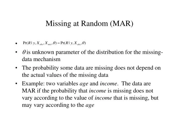
1. Missing at Random (MAR) •  is unknown parameter of the distribution for the missing-data mechanism • The probability some data are missing does not depend on the actual values of the missing data • Example: two variables age and income. The data are MAR if the probability that income is missing does not vary according to the value of income that is missing, but may vary according to the age

2. Missing Completely at Random (MCAR) • The probability some data are missing does not depend on either the actual values of the missing data or the observed data • The observed values are a random subsample of the sampled values • Example: The data are MCAR if the probability that income is missing does not vary according to the value of income or age

3. Dealing with Missing Features • Assume features are missing completely at random • Discard observations with any missing values • Useful if the relative amount of missing data is small • Otherwise should be avoided • Rely on the learning algorithm to deal with missing values in its training phase • In CART, surrogate splits • In GAM, omit missing values when smoothing against feature in backfitting, then set their fitted values to zero (amounts to assigning the average fitted value to the missing observations)

4. Dealing with Missing Features (con’t) • Impute all missing values before training • Impute the missing value with the mean or median of the nonmissing values for that feature • Estimate a predictive model for each feature given the other features; then impute each missing value by its prediction from the model • Multiple imputations to create different training sets and access the variation of the fitting across training sets (e.g. if using CART as imputation engine, the multiple imputations could be done by sampling from the values in the corresponding terminal nodes)

5. Questions about Missing Data • For the missing data, I still want to ask the question i asked in last email, can we have a generalization of the missing data handling for different methods? [Yanjun] • p. 294, it's not clear for me how you go about doing imputation, since we still face the same problem of partial input when predicting the missing feature value from the available ones, i.e., each time a different set of features are available to predict the missing ones. [Ben]

6. Linear Model Generalized Linear Model Additive Model Generalized Additive Model Regression Models

7. Smooth Functions fj(•) • Non-parametric functions (linear smoother ) • Smoothing splines (Basis expansion) • Simple k-nearest neighbor (raw moving average) • Locally weighted average by using kernel weighting • Local linear regression, local polynomial regression • Linear functions • Functions of more than one variables (interaction term)

8. Questions about Model • In pp. 258, the authors stress that each f_i(X_i) is a "non-parametric" function. However, in the next few sentences, they give examples to fit these functions with cubic smoothing splines, which assume the underlying models. It seems these two statements are contradictory. The other question is whether parametric or non-parametric functions is more appropriate in the generalized additive models. [Wei-Hao] • From the reading it seems to me that the motivation to use GAM is to allow "non-parametric" functions to be added together. However, these are simply smoothed parametric basis expansions. How is this "non-parametric" and what has this gained? [Ashish] •  I tried but failed to figure out why the minimizer for generalized linear additive model is additive cubic spline model. Any clues? We don't have to assume any function forms for those f_i(x_i)? [Wei-Hao] • Since the minimizer of Penalized Sum of Squares (Eq. 9.7) is additive cubic splines, what are justifications to use other smoothing functions like local polynomial regression or kernel methods? [Wei-Hao]

9. Questions about Model (con’t) • I have noticed formula 9.7 in P259. In order to guarantee the smoothness, we simply extended our method from one dimension to N dimension using \sum f_j''. But this can only guarantee the smoothness on each single dimension and can not guarantee the smoothness on the whole feature space. It is quite possible that on every dimension the function is very smooth but There are much bumpy "between dimensions". How can we solve it? Is this a shortcoming of backfitting? [Fan] • It appears to be the case that, to extend the generalized additive model such as considering the basis function with several variables will be quite messy. Therefore, even though, the additive model is able to introduce the nonlinearity into the model, it still lacks the strong ability of introducing the nonlinear correlation between inputs into models. Please comment it by comparing to the kernel function. [Rong]

10. Fitting Additive Model • Backfitting algorithm • Initialize: • Cycle: j = 1,2,…, p,…,1,2,…, p,…, (m cycles) Until the functions change less than a prespecified threshold • Intuitive motivation for the backfitting algorithm • If additive model is correct, then • mp applications of a one-dimensional smoother, NlogN+N operations for cubic smoothing splines

11. Fitting logistic regression (P99) Fitting additive logistic regression (P262) 1. where 1. 2. 2. Iterate: Iterate: a. a. b. b. c. Using weighted least squares to fit a linear model to zi with weights wi, give new estimates c. Using weighted backfitting algorithm to fit an additive model to zi with weights wi, give new estimates 3. Continue step 2 until converge 3.Continue step 2 until converge

12. Model Fitting • Minimize penalized least squares for additive model or maximize penalized log-likelihood for generalized additive model • Convergence not always guaranteed • guaranteed convergence under certain conditions – see Chapter 5 of Generalized Additive Model • converge in most cases

13. Questions about Fitting Algorithm • It seems to me that the ideas of "backfitting" and "backpropagation" are quite similar to each other. What makes different? Under what condition will Gauss Seidel converge? (linear & nonlinear system) And how fast? [Jian] • For the local scoring algorithms for additive logistic regression, can we make a comparison with the page 99 which is about fitting logistic regression models? [Yanjun] • Could you explain the algorithm 9.2 more clearly? [Rong] • On p. 260, by stipulating that Sum_{i=1..N} f_j(x_{i,j})=0 for all j, do we effectively the variance over training sample to be 0? (note alpha in this case is avg(y_i) ) Why do we want to do that? What's the implication to the bias? [Ben]  • In Page 260, for the penalized sum of squares, for (9.7), if the matrix of input values is singular (uninvertible), the linear part of the f_j can not be unique, but the nonlinear part can be ... what and why does this happen? [Yanjun]

14. Pros and Cons PRO: • No rigid parametric assumption • Can identify and characterize nonlinear regression effects • Avoid curse of dimensionality by assuming additive structure • More flexible than linear models while still retaining much of their interpretability CON: • More complicated to fit • Have limitation for large data-mining applications

15. Where GAMs are Useful • The relationship between the variables is expected to be of a complex form, not easily fitted by standard linear or non-linear methods. • There is no a priori reason for using a particular model • We would like the data to suggest the appropriate functional form • Explanatory data analysis

16. Questions about Link Functions • For GAM, the books gives us three examples of the link functions and points out that they are from exponential family sampling models, which in addition includes gamma and negative-binomial distribution. Can we find out why we use these kinds of functions as link functions? [Yanjun] • Can you explain to me about the intuition of the classical link functions, how each function corresponds to one particular data distribution as is said on page 258? That is, g(x) = x corresponds to Gaussian response data, logit to binomial probabilities, g(x)=log(x) for Poission count data? [Yan]  • On p. 259 various possibilities in formulating the link function g are mentioned. Could you hint at how we actually come up with a particular formulation? By correlation analysis? Cross validation? [Ben]