Download
1 / 54
570 likes | 712 Views
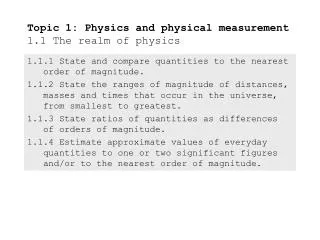
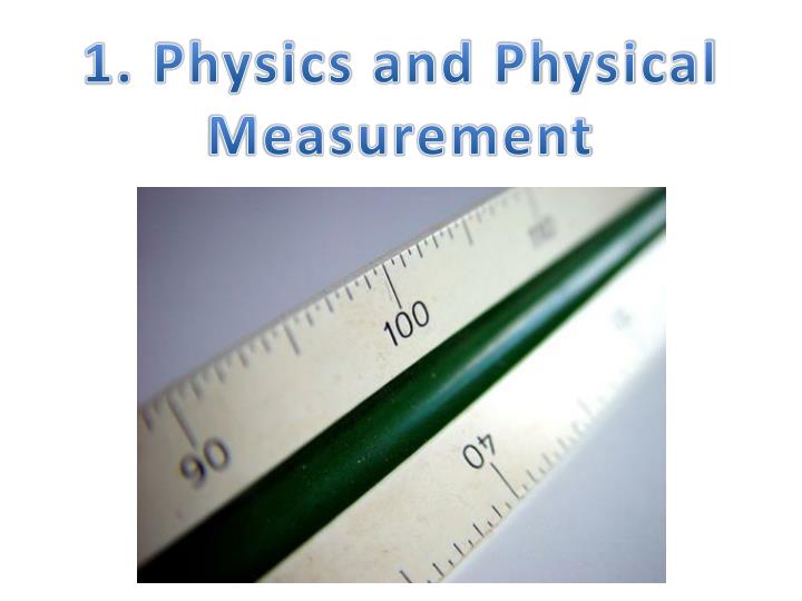
1. Physics and Physical Measurement. Topic Outline. The skills in this section are important for your internally-assessed lab reports The graphing skills in this section are important for Paper 2, Section A. Orders of Magnitude.

E N D
Topic Outline • The skills in this section are important for your internally-assessed lab reports • The graphing skills in this section are important for Paper 2, Section A
Orders of Magnitude Metric prefixes are used to express large or small numbers in a form that is more manageable
Standard Form • In standard form, we write one digit before the decimal place and then the appropriate order of magnitude 476 293 000 = 4.76293 x 10⁸ 0.000000516 = 5.16 x 10⁻⁷ • Orders of magnitude can be used to estimate or compare measurements
Significant Figures Significant figures are digits that are not merely placeholders
Significant Figures Significant figures are digits that are not merely placeholders
Rounding • Calculations are rounded to the same number of significant figures as the least accurate value in the calculation 2.430923485498 + 3.1 = 5.5 (2 s.f.)
Exercises • Worksheet 1: Significant figures and standard form
SI Base Units • Physicists have an agreed system of units, called ‘Le Système International d’Unités’ (S.I. Units) • There are seven base units, all other units are derived from these
Derived Units • Derived units are formed from a combination of SI base units • To derive a unit for a variable, we use the equation for that variable F = m x a So the units for force are kg x ms-2 = kgms-2 = N Note: you must use negative index notation for units, e.g. use ms-2not m/s2
Standard Measures • A standard measure is used as a reference • It must be: • Unchanging with time • Readily accessible • Reproducible The standard second is the time for 9 192 613 770 vibrations of the cesium-133 atom
Errors • Errors are sources of uncertainty in a measurement • There are two main classes of error: • Systematic errors are the result of the equipment or method (system), e.g. zero error, poorly calibrated instruments • Random errors occur randomly and are reduced by repeating measurements, e.g. normal variations, parallax error, insensitive instruments
Accuracy and Precision • Accuracy is an indication of how close a value is to the true value (how close it is to the bull’s eye) • Precision is an indication of how similar repeated measurements are (the ‘grouping’ of shots at a target)
Uncertainties • The uncertainty is an estimate of the possible inaccuracy in a measurement • We estimate the uncertainty in a measurement to be half the ‘limit of reading’, i.e. half the smallest scale division • If there is possibility for error at either end of the measurement, the uncertainty is the smallest scale division • If repeated measurements are made, the uncertainty is half the range of the measurements • Uncertainties are given to 1 s.f. only
Practical • Observe zero error with a force meter • Observe parallax with an analogue meter • Time one oscillation of a pendulum then compare with measuring 10 oscillations and dividing by 10 • Use Vernier calipers to measure the thickness of a piece of paper • Use Vernier calipers to measure the diameter of a marble, make 5 measurements to give a value and an uncertainty
Exercises • Worksheet 2: Uncertainties • Giancoli pp. 16-17 (section 1.4, 1.5-1.7)
Absolute and Percentage Uncertainties • The absolute uncertainty is given in the same units as the measurement • The percentage uncertainty is expressed as a percentage of the measurement 2.3 ± 0.5 cm = 2.3 cm ± 20%
Combining Uncertainties • When adding or subtracting measurements, add the absolute uncertainties • When multiplying or dividing measurements, add the percentage uncertainties • When raising a value to a power, multiplythe percentage uncertainty by the absolute value of the power
Practical • Measure the volume of a coin • Process your uncertainties to give an uncertainty with the final measurement
Exercises • Worksheet 3: Combining uncertainties
Graphing Skills • When drawing a graph: • Use pencil, ruler and graph paper • Use suitable sized axes • Mark values with a linear scale • Label the axes, including units • Give a descriptive title • Plot data points • Draw a best-fit trend line
Graphing Skills • To find the gradient: • Find two places where the best-fit line passes through easy-to-read points on the graph • Calculate the rise (Dy) • Calculate the run (Dx) • Calculate the gradient (Dy/Dx)
Graphing Skills • To graph uncertainties: • Error bars are used to represent uncertainties in a measurement • The uncertainty in the y-value is drawn vertically • The uncertainty in the x-value is drawn horizontally • The best-fit line is the line that best represents the data • The error line is the steepest (or least steep) line that can be drawn through the error bars
Graphing Skills • Interpolation is finding a value between plotted points • Extrapolation is finding a value beyond plotted points
Linear: y a x • If the y-intercept is zero, we can also say that y is directly proportional to x
Squared: y a x2 • Plotting distance vs. time2 will give a straight line graph of the form y = mx + c
Squared: y a x2 d = 5t2 + 0 y = mx + c
Square Root: y a√x • Plotting time vs. √distance will give a straight line graph of the form y = mx + c
Inversely Proportional: y a 1/x • Plotting volume vs. 1/pressure will give a straight line graph of the form y = mx + c
Inverse Square: y a 1/x2 • Plotting intensity vs. 1/distance2 will give a straight line graph of the form y = mx + c
Sinusoidal • Sine and cosine graphs; these will be covered more in Topic 4
Exponential (AHL): y a ex Exponential decay of a radioactive sample N = N0e-kt
Exponential (AHL) • Taking the natural log of both sides gives lnN = lnN0 + lne-kt lnN = lnN0 - kt lnN = -kt + lnN0 • Plotting lnN against t gives an equation of the form y = mx + c, with a gradient of –k and a y-intercept of lnN0
Exponential (AHL) lnN = -kt + lnN0
Logarithmic • Don’t yet have a good example, sorry
Exercises • Graphing Relationships (Rutter pp. 13-27)
Vectors and Scalars • Scalar quantities only have magnitude (size) • e.g. distance, speed, mass, time,, charge, energy • Scalars are added algebraically • Vector quantities have magnitude and direction • e.g. displacement, velocity, force, momentum • In IB, a vector is represented in bold, italicised print • Vectors are added in a particular way
b a a b a +b Vector Addition • Vectors are added ‘head to tail’ to find the resultant vector • For example, adding vectors aand b • If this forms a right-angled triangle, use Pythagoras’ Theorum to find the length of the resultant, and trigonometry to find the angle
b -b a - b a -b a Vector Subtraction • To subtract one vector from another, switch the direction of the arrow of the vector that is to be subtracted, then add the vectors • For example, a - b
3a a Multiplying a Vector by a Scalar • To multiply a vector by a scalar, keep the direction of the vector the same and multiply the magnitude by the scalar • For example, 3 x a
Multiplying Two Vectors (AHL) • The dot product is when two vectors are multiplied to give a scalar • For example W = F x d • Work is a scalar, but force and displacement are vectors • Work is calculated by W = F . d = |F| x |d| x cosq • Where q is the angle between F and d
Multiplying Two Vectors (AHL) • The cross product is when two vectors are multiplied to give another vector • For example, F= qvB • Force, velocity and magnetic field strength are all vectors (charge is a scalar) • The cross product vB is calculated vB = |v| |B| sinq • Where q is the angle between F and d • The direction of the resultant is at right angles to both v and B, given by the right-hand-thumb rule
X- and Y-Components of a Vector • A vector can be resolved into its horizontal and vertical components • We use trigonometry to find the lengths of the x- and y-components
Exercises • Giancoli p. 70-71 (sections 3.2-3.4)
Revision • Questions from Paper 2, Section A • Practice internal – Simple Pendulum