Download
1 / 18
180 likes | 340 Views
Directed Acyclic Graphs: A tool to incorporate uncertainty in steelhead redd -based escapement estimates. Danny Warren Dan Rawding March 14 th , 2012. Outline. Coordinated Data Assessments Project What’s a DAG? Mill, Abernathy, Germany monitoring history. Redd Estimates. Using DAGs.

E N D
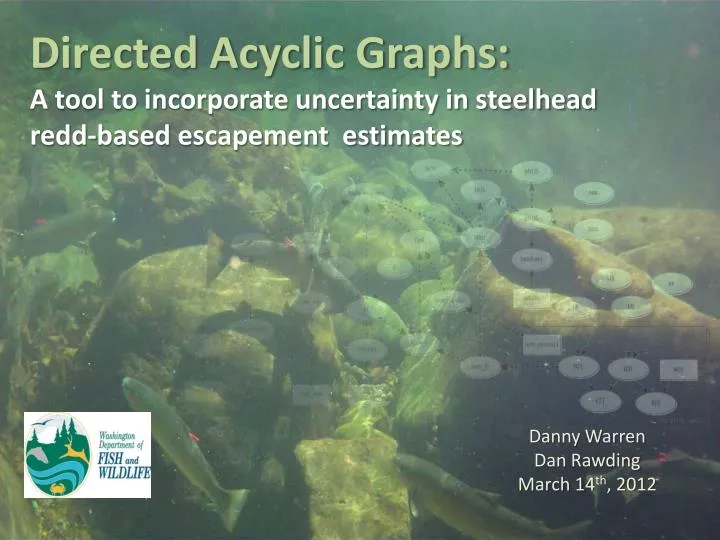
Directed Acyclic Graphs: A tool to incorporate uncertainty in steelhead redd-based escapement estimates Danny Warren Dan Rawding March 14th, 2012
Outline • Coordinated Data Assessments Project • What’s a DAG? • Mill, Abernathy, Germany monitoring history Redd Estimates Using DAGs Escapement Estimates
Coordinated Data Assessments • Broad effort across numerous Columbia Basin entities • Goal to improve data timeliness, reliability, and transparency • Focused on 3 high-level indicators: • Natural Spawner Abundance • Smolt to Adult Ratio • Recruits per Spawner Needs identified: • Improved data infrastructure • Better documentation • Standardized analytical methods
So what’s a DAG? • Graphical representation of a statistical model • Explicitly depicts the data, equations, and statistical distributions • Easy to translate into code or statistical nomenclature • Accounts for all uncertainty in indicator estimates SIMPLE DAG HEREA DAG for % Female a_LB a_UB b_LB b_UB pred_pF a b pF[i] females[i] adults[i] For(i IN 1 : sex_obs)
Bayesian Approach for Redd Estimates • PosteriorProbability ~ Likelihood * Prior Distribution • Does not rely on normal distribution • Yeilds similar results to maximum likelihood as long as priors are vague. • Hierarchical modeling allows sparse or missing data borrow strength from other data Age data from Toutle River Fish Collection Facility
Redd-Based Escapement Estimate • Define Sampling Frame or Universe (potential spawning dist.) • Representative sampling design (SRS,GRTS,SYS,etc) • Estimate the redddenisty • Use goodness of fit (GOF) tests to check if the observed density fits the model • Total Redds= Obsredds + (redd density * unsurveyed distance) • Adults = Total redds • NOS = (1-pHOS) * Adults • Adults[age] = Adults * % by age Females per redd * % Female
Redd Survey Design 2005-2011 • Census on mainstems and some tributaries • One reach with landowner conflict • Several supplemental reaches near peak
Redd Survey Design 1994-2004 • Systematic approach to establish index reaches surveyed throughout season • Supplemental reaches surveyed near peak • Redd density expanded to unsurveyed reaches • No surveys or estimates in Mill Creek
Steelhead Redd Locations • Redd locations are clumpy! • Some reaches have few redds. • Others have many, especially below the hatchery.
Goodness of Fit Bayesian p-value tests how well model fits observed data p of 0.50 = Best fit p of 0 or 1 = Poor fit Summary of years 1994-2011
WinBUGS Output • Also a text file with: • Mean and median • Standard deviation • 95% CI • Sample iterations
Total Redds Implementation of census surveys No error for complete census surveys!
Patterns and Variability • Redd data in this basin follows a negative binomial distribution (not normal) in part due to hatchery effects. Increasing uncertainty NOAA has proposed CV < 15% of escapement Greatest sources of variability: Females per Redd estimate CV = 13.5% Sampling design CV = 14-33% pNOSCV >25%
Discussion • There is a need for greater transparency and documentation of redd-based abundance estimates • Census survey design is ideal, but stratified sampling of high and low density areas would also lead to precise estimates • Hierarchical modeling is an effective tool for time-series data with gaps or limited data
Questions? Photo : Steve VanderPloeg