Download
1 / 20
300 likes | 2.1k Views
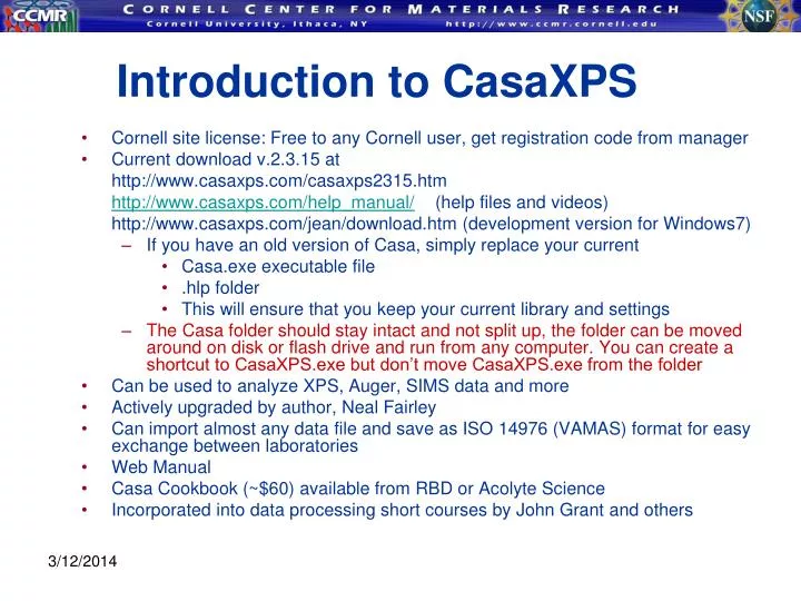
Introduction to CasaXPS. Cornell site license: Free to any Cornell user, get registration code from manager Current download v.2.3.15 at http://www.casaxps.com/casaxps2315.htm http://www.casaxps.com/help_manual/ (help files and videos)

E N D
Introduction to CasaXPS • Cornell site license: Free to any Cornell user, get registration code from manager • Current download v.2.3.15 at http://www.casaxps.com/casaxps2315.htm http://www.casaxps.com/help_manual/ (help files and videos) http://www.casaxps.com/jean/download.htm (development version for Windows7) • If you have an old version of Casa, simply replace your current • Casa.exe executable file • .hlp folder • This will ensure that you keep your current library and settings • The Casa folder should stay intact and not split up, the folder can be moved around on disk or flash drive and run from any computer. You can create a shortcut to CasaXPS.exe but don’t move CasaXPS.exe from the folder • Can be used to analyze XPS, Auger, SIMS data and more • Actively upgraded by author, Neal Fairley • Can import almost any data file and save as ISO 14976 (VAMAS) format for easy exchange between laboratories • Web Manual • Casa Cookbook (~$60) available from RBD or Acolyte Science • Incorporated into data processing short courses by John Grant and others
Introduction to Data Analysis • File formats (text, Vamas, etc.) • Background subtraction (Shirley, linear, Tougaard) • Identifying elements • Quantitative analysis • Peak fits (Gaussian-Lorentzian, Voigt, Doniach-Sunjic) • Atomic % (tags) • Chemical shifts • Propagating analysis to multiple data sets • Backgrounds • CasaXPS software • Display data • Report generation • More
Importing/Exporting Data • Exporting text Files (for Excel or other program): • Highlight the blocks to be exported and click: • ‘Save Tab ASCII’, when asked ‘export as column of tables?’ click ‘yes’ to get two long columns of data, or ‘no’ to get multiple pairs of columns. • ‘Save Tab ASCII to clipboard’ • Can also save in Quases format for Tougaard analysis Importing Vamas Files: • Acquisition parameters (# scans, pass energy, date, time, etc.) are contained in the Vamas file • Just double-click the Vamas file and CasaXPS will open • Ignore any SSI quantification error on opening • Click “EDIT MODE” to see any sample labels or original file names • Can also use the File---Open and Merge command to combine multiple Vamas files • Click on the ‘? Edit sample ID’ icon to change any names or SampleIDs of highlighted blocks • ‘Intensity Calibration’ or the transmission function should automatically be -0.7 for data taken on the SSI system. • Importing Text Files (must rename to .dat): • Go to File, Convert and CasaXPS will read in all text files in the folder • # of scans will be assumed to be 1. This can be changed manually in the Block Info. Use caution when comparing data sets with different: • # of scans • Dwell times • Resolution • For SSI text data make sure the ‘Intensity Calibration is -0.7 by clicking the Quantity(F7) icon
File Handling • Click “EDIT MODE” to see any original file names • FG means Flood Gun was used for charge compensation • FGG means the Flood Gun and Grid were used for charge compensation • _0, _30, _55, e.g. refer to the emission angle for ARXPS. _0 is the sample normal (deepest analysis). If no angle is given 55-degrees is assumed. • You may edit the blockID or sampleID by clicking on the “?” icon to the left of EditMode • Can rename species and transitions as well • If rows are not already arranged, select all blocks in a row and click ‘edit by row’ • Choose a variable label (e.g. sample, time, depth, etc.) • Choose a variable value higher than the # of blocks you have. • Repeat to sort each block into its label# • Blocks should be sorted into columns by peak transition • Using the ‘species/transition’ icon, label the element and transition (survey, Au 4f, C 1s, e.g.) • Or, open the element Library(F10) • Click on your peak to narrow the element table down • Select your peak/transition (C1s, Au4f, Au 4f 7/2, etc. ) • Click ‘edit Block Species/Trans’ • Click OK and your data block will go under its own column (C1s, Au4f, etc. ) • Clicking the trash-can ‘delete Vamas blocks’ will delete all highlighted blocks (cannot undo) • Clicking the clipboard for ‘copy/paste Vamas blocks’ will add all highlighted blocks into the current data set. Even blocks from other Vamas files can be copied if highlighted. • Spectra can be copied to the clipboard or saved as an EMF • Data is saved in Vamas format
Displaying Data Display(F1) Page Layout(F5) Zoom In Reset(F4) Overlay(F2) Display Parameters(F6) Zoom Out(F3) • By highlighting blocks and clicking ‘display’ (F1), each block will be displayed separately. Scroll down to see other spectra • By highlighting blocks and clicking ‘overlay’ (F2), to compare similar data • By clicking-and-dragging a box on your spectrum, then pressing ‘insert’ on your computer’s keyboard, an inset will be made. Highlight the block to inset and click ‘Overlay’(F2). • Insets can be edited the same way as other displayed spectra • You can make insets within insets • Delete the inset by clicking on it and pressing ‘Delete’ on your keyboard • Use ‘Page Layout(F5)’ to save or pick from 16 different tile formats. Tile format files can be saved or loaded • Use ‘Display Parameters(F6)’ to adjust color, fonts and other parameters. This can be saved as well in the ‘Global’ tab • The BE/KE icon switches data between KE and BE • The CPS/C icon switches data between count rate(CPS) and total counts. • Note: CasaXPS uses CPS to calculate data, not counts! (i.e. increasing the number of scans should affect the analysis only by making the data smoother, with greater signal-to-noise ratio)
Survey Scan Analysis • Open the ‘Library’(F10) • Select elements using the periodic table or element table • Click ‘create regions’ and default regions with peaks will be created • If the peak is selected in the Element table, the region will have the peak name (Au4f e.g.) • Zoom in on individual peaks and adjust regions using the ‘Quantify’(F7) icon • Atomic% will be adjusted accordingly • Some regions may need to be added manually • By default, CasaXPS will look for the peak with the greatest RSF value • In the case of a doublet, CasaXPS may assign a doublet region to a single peak • To change the default peak, open the CasaXPS_quant.lib file and add/replace the peak transition you prefer, from CasaXPS.lib
Regions and Backgrounds • Open the Library(F10) and select your peak in the Element Library • Open the ‘Quantify’(F7) box • Click Create Region • Adjust blue area to your peak(s) • BG Type will be Shirley by default • Can type S for Shirley background • ‘L’ for linear. Typically works well for polymers • ‘OS’ for offset Shirley (combined linear/Shirley, only works in v.2.3.13). May work for doublets • In the field ‘Cross Section’, the last 2 values adjust the proportion of linear to Shirley and the offset • 0, 0, 0.4, 5 would mean a 40% linear(60%Shirley) with a 5 eV offset • ‘T’ for Tougaard • Av Width, value n, can be used to smooth endpoint • Will use the average height of 2n + 1 data points • Shirley backgrounds are generally good for metal XPS peaks • intended for single peaks • Can use 2 separate regions to describe a doublet • Can put 2 regions in one plot, but regions cannot overlap • Must use caution with backgrounds in general as it will have a large effect on the analysis • Consistency may be most important
Peak Shapes • CasaXPS default peak shape is GL(30) which is intended for Kratos systems • GL(15) should provide closer fits to data from SSI systems • To change the default, find the file CasaXPS.lib in your Casa folder • Open with Excel and change the whole GL(30) column to GL(15) • GL(x) is a Gaussian-Lorentzian peak shape with x being the % Lorentzian • GL(0) is 100% Gaussian. Analyzer resolution is Gaussian • GL(100) is 100% Lorentzian. X-ray lines are Lorentzian • May need to adjust GL value depending on whether lineshapes are analyzer or x-ray limited • LA is an asymmetric new to the 2.3.14 version of Casa Purple: Gaussian Blue: Lorentzian same peak areas
Shifting Data • Processing (F8) can be used to shift data • Click on the ‘Calibration’ tab • Click on your peak and a Measured energy will appear • Type in the true intensity and click ‘Apply’ • Can be applied to Regions and Components by checking boxes • Note: • SSI system is calibrated to Au4f at 84/88eV • CasaXPS defaults to 83/87eV • Can go into the CasaXPS.lib file and change the Au4f7/2 to 84eV and Au4f5/2 to 88eV • Can reverse data shifts by clicking on the ‘Processing History’ tab and removing any commands
Peaks/Components: Fitting Data • Note: It will help if your block Species/Transition is named correctly, or the default lineshape will be GL(30) instead of what you have in the library • Create a region around your peak(s) • Click the ‘Components’ tab • Click ‘Create Component’ • If the peak is selected in the Element table, the component will have the peak name (Au4f7/2 e.g.) • Can also type in “# Au 4f 7/2” in the ‘Name’ field to bring up the library RSF value • When you click on a peak, you can: • See the residual at the top, in black, which you would like to be flat when fit well. The next created peak will be inserted where the largest negative residual lies. • Drag the top of the peak to change Area and Position • Drag the side of the peak to change FWHM • Repeat for # of components you need • Click ‘Fit Components’ to obtain a fit to the data • Components can be removed by selecting and clicking ‘Cut’
Spin-Orbit Splitting • Very subjective • Can use two separate regions to define both peaks • Can use a Shirley/linear background (v.2.3.13 only) • Type ‘OS’ into region background field • Can use a linear background • Can constrain peak areas to theoretical values
Constraints (components) • Can create Component Constraints: • In the component fields, make sure you press enter, don’t click after entering a value • Position (eV) • Known chemical shifts • Can set X,Y in the constraints field where X is lower limit and Y is upper limit • A+1.2 means 1.2 eV higher than position of peak A • FWHM • May vary with transition or chemical shift • Area • 4f 7/2 peak area should be 4f5/2 area*1.3333 (4:3 ratio) • 3p 5/2 = 3d 3/2 *1.5 (3:2 ratio) • 2p 3/2 = 2p 1/2 *2 (2:1 ratio) • A*1.333 would constrain the peak to 1.333 times the area of peak A
Displaying Component Table • Each component can have a unique Name • Open the ‘Tile Annotation’(F9) box • Click the Quantification tab • Can click the Components tab if only comparing components • Can click the Regions tab for comparing regions • Click table type for components, regions, or both • Click ‘Apply’ • Annotation History • Can move the table by click and dragging the red box that appears • Can remove the table by deleting the annotation history line
Report Generation • Standard reports provide areas/atomic%, FWHM, BE’s, etc. that you can export as a text file • Highlight the blocks that you want included in the report • Open the ‘Quantify’(F7) icon • Click on the ‘Report Spec.’ tab • In the Custom Report window, highlight the regions and components needed, or click ‘all’ • By clicking Area Report, a text file will be generated with associated data • Custom reports can provide ratios with respect to one element • In ‘Custom Report’ click on Regions or Comps depending on what you have • Select a region/component to compare everything else to • Click ‘Ratio Region’ or ‘Ratio Comp’ • The formula will appear below for what is being ratio’ed • Click ‘Area Report’ to get the ratios and %’s • The text files can be saved and imported into another program (Excel, Origin, etc.)
Inserting Text • Click the pencil for ‘Annotation’(F9) • Click the ‘Text’ tab • Type in your text, check the ‘Draw Line’ box if needed • Click ‘Apply’, your text will appear • Click Annotation History • A red box will appear which you can use to move the text • Font size can be changed • Unwanted lines can be deleted • Text will stay with the primary block
Advanced: Propagating Analyses • You can propagate the following analyses: • Regions • Components • Processing and more • Careful propagating too much • Bring up the spectrum you would like to propagate • Highlight the blocks you would like to propagate to • Either right-click the spectrum, OR click the ‘Propagate to Selection’ icon • Your selected blocks should appear and allow you to choose what you would like to propagate (regions, components, processing, annotation, etc.) • Selected spectra will have parameters applied
Advanced Quantitative Analysis • Peak scans can be displayed along with survey scan data • Similar to example on p.113 of the Casa Cookbook • All data sets must be taken at Resolution4 (if different step sizes, may need to adjust for this) • Blocks must be in the same row • In ‘Annotation’(F9), click quantification • Click ‘Table Type Regions’ • Click ‘Apply’
Advanced Components: Tags • Component Tag field must be identical to the tagged Region field (in the survey scan, e.g. ) • Highlight the blocks of interest • Open ‘Annotation’(F9) • Click the Quantification tab • Click table type for components • Click ‘Use Tag Field’ • Click ‘Apply’ • Component %’s will total up to the tagged atom%
Overlayer Effects • Copper thin film on gold • Heterogeneous structure • Buried thick copper layer between gold • Copper substrate beneath gold
Overlayer Effects • A pure gold sample would show equal atomic% for all peaks • An overlayer will cause the lower KE (higher BE) peaks to be reduced in area • The data here indicate a Carbon overlayer (C peak at 284 eV) that is attenuating the Au peaks at higher BE’s