Download
1 / 25
250 likes | 356 Views
Scatterometer Algorithm. July 19, 2010 Seattle. Simon Yueh , Alex Fore, Adam Freedman, Julian Chaubell Aquarius Scatterometer Algorithm Team. Outline. Key Requirements Technical Approach Algorithm Development Status L1A-L1B L1B-L2A Post-Launch Cal/Val Plan

E N D
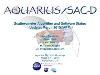
ScatterometerAlgorithm July 19, 2010 Seattle Simon Yueh, Alex Fore, Adam Freedman, Julian Chaubell AquariusScatterometer Algorithm Team
Outline • Key Requirements • Technical Approach • Algorithm Development Status • L1A-L1B • L1B-L2A • Post-Launch Cal/Val Plan • Remaining Issues and Plans
Key Scatterometer Algorithm Requirements Produce geolocated, calibrated normalized radar cross-sections (Sigma0) Locate each Sigma0 on Earth. Convert the L1A Aquarius data from counts to calibrated normalized radar cross-sections (Sigma0) Generate an error estimate (Kpc) for Sigma0. Incorporate quality control flags (RFI, land fraction, etc) Generate ocean surface wind speed estimates for corrections of surface roughness effects on Tb
Technical Approach • Develop scatterometer simulator for end-to-end data processing system testing and post-launch cal/val tool development. • The simulator will be updated and used as a testbed to develop new algorithms. • Algorithm/software will be modularized to allow plug and play. Ephemeris, Attitude Instrument parameters Ancillary fields Geophysical Model Function Scatterometer telemetry simulator L1A Simulator Science Data Processing System L1A Reader L1A-L1B Processor Reader Instrument parameters Ancillary fields L1B Reader Scatterometer L2 Processor Radiometer Faraday rotation Ancillary fields Geophysical Model Function Reader Simulator and AlgorithmTestbed
L1A to L1B Algorithm Structure Read ephemeris/attitudes. Compute cubic splinecoeffs. L1A Input file Input flags Info/Debug files Read radar science data. Read instrument telemetry. Quality check of data. Compute look vectors. Compute LB-corrected echo power into antenna. Compute SNR, Kpc. Use K-factors to compute geolocated sigma-0. Compute land, ice fractions. Compute flag info. Write L1B Output. K-factor tables.Land mask. To L2 processing Antenna patterns (6) Sea ice data HDF-4 Level 1B File (includes processing flags) Instrument parameters
Level 1 ATBD (Calibration Equation) Antenna pattern and radar equation Electronics cal (Cal loop&losses) Noise Subtraction Radiometric cal • Ps= signa+noise data, Pn=noise only data and Pcal= cal-loop data. It is very time consuming to carry out the 2-d numerical integration (Xint) for all orbit steps and attitude Impractical for in-line data processing
K-factor and Radiometric Calibration • K-factor will be a look-up table with 4 parameters: beam#, polarization, latitude and incidence angle, rather than 7 parameters • The difference between full scalar radar equation integration and K-factor approximation is < 0.01 dB
Key Characteristics and Content of L1B data File • A special Cal/Val product – not planned for routine production • Data block at 1.44 sec interval • S/C position and attitude • Latitude and longitude of footprint center and corners • Radar quad pol (VV, HH, VH and HV) data at 0.18 sec interval • Incidence and azimuth angles • Measurement uncertainty (kpc) • Land fraction: fraction of land surface weighted by antenna gain • Ice fraction: fraction of sea ice weighted by antenna gain • RFI flag
Baseline L1B-L2A Processing Flow L1B geolocated, calibrated TOI σ0 Average over block; filter by L1B Qual. Flags L2A (lon, lat) L2A σTOI+ KPC • Ancillary Data: • ρHHVV,fHHHV, fVVHV • ΘF (from rad or IONEX) L2A σTOA+ KPC Cross-Talk + Faraday Rotation Wind Retrieval L2A wind + σwind • Ancillary Data: • -PALS 2009 Model Function • Ancillary Data: • NCEP wind dir. ΔTB retrieval L2A ΔTB+ σΔTB
Cross-pol/Faraday Rotation Correction Beam 3 • The algorithm using the antenna pattern and faraday rotation data significantly reduces the error of each polarized VV, HH, VH and HV sigma0s. (<0.1 dB for strong backscatter) • See Alex Fore et al’s paper for details of the correction algorithm No correction With correction No correction With correction
L2A Wind Retrieval Process Flow Baseline algorithm: -total σ0 approach. -Faraday rotation and cross-talk has no effect on total σ0 approach. Ancillary Inputs: -NCEP wind direction Inputs: -Total σ0 -antenna azimuth -Kpc estimate L2A Scat wind speed + error Solve for wind speed Newton’s Method: 1d root-finding problem Newton’s Method Aquarius ScatterometerModel Function (PALS 2009) -input: wind speed, relative azimuth angle, incidence angle (or beam #) -output: total sigma-0
Simulated Total σ0 Wind Retrieval Performance • Total σ0 performance is independent of any Faraday rotation corrections or cross-talk removal. • As compared to beam-center NCEP wind speed: • Wind Speed B1 std: 0.205 m/s • Wind Speed B2 std: 0.186 m/s • Wind Speed B3 std: 0.226 m/s • By construction, when we derive the model function from the data there will be no bias.
Scatterometer Performance Simulation Radar sigma0 simulation (weekly for 2007) Wind speed estimate simulation (weekly for 2007)
L2A ΔTB Estimate • L2 ΔTB will be the scatterometer wind speed times the PALS dTB/dw. (Note: not included in v1 delivery) • We estimate the ΔTB errors due to the wind RMSE numbers. • The simulated sd error is about 0.05 K for vertical polarization and 0.07 K for horizontal polarization, better than the 0.28K allocation PALS Tb relation:
Key ScatterometerProdcuts in L2A • Average over 1.44 sec • TOI Radar Sigma0 (VV, HH, VH and HV) • TOA Radar Sigma0 (VV, HH, VH and HV) • Scatterometer wind speed and expected standard deviation • TBV and TBH corrections and expected standard deviation • Scatterometer land fraction – not the same as radiometer land fraction • Scatteroemter sea ice fraction – not the same as radiometer ice fraction
Post-Launch Cal/Val Conceptual Plan • Telemetry Analysis • Time series of system noise, temperature, voltage and current • L1B analysis • Pointing angle analysis using sigma0 changes along land/sea crossings • Sigma0 Calibration stability • Time series of radar sigma0 over distributed targets (Antarctic, Dome-C, Amazon, Greenland) • Global ocean sigma0 histogram vs time • Faraday rotation analysis (comparison with modeling analysis using IONEX and IGMF B fields) • L2 analysis • Sigma0 geophysical model function (Aquarius, NCEP wind, SST, and wave matchup) • Sigma0-TB geophysical model function (Aquarius, NCEP, SST, and wave matchup)
Model Function Development Methodology • Process all 2007 data to level 2. • Collocate simulated scatterometerσtot observations with NCEP wind vectors. • Filter observations with non-zero land/ice fractions. • Use NCEP data that is offset by 6h from simulated scatterometer observations. • 6h as compared to 0h: rmsspd diff: 1.9 m/s; rms dir diff: 27.5 deg. (computed @ beam center) • Average NCEP winds over beam footprint. (Not done for these results).
Model Function for Beam 1 Cosine Series (6h offset) • Need probably 3 months of data for convergence for <20 m/s wind speed. • The error caused by noisy matchup needs to be resolved.
Experimental Wind Retrieval Process Flow Ancillary Inputs: -SST Inputs: -VV, HH, HV and VH σ0 -TBV, TBH -cell azimuth, incidence angle Wind Speed and Direction Solutions Minimize LSE for wind speed and direction Search for local minimma ScatterometerModel Function (PALS 2009) Radiometer Model Function -input: wind speed, relative azimuth angle, incidence angle (or beam #) -output: sigma-0 and TB
Wind Vector Estimate Using VV and TH Distinct characteristics of TB and Sigma0 will allow the estimate of wind speed and direction. The RMS differences between PALS (closest solution) and POLSCAT winds are 1.4 m/s and 15 deg. Wind speed and direction solutions derived from PALS radiometer TH and radar σVV data are illustrated versus the ocean surface wind speed and direction derived from the POLSCAT Ku-band measurements acquired on 26 February, 2 March and 5 March 2009. In general, the single azimuth look observations will allow four directional solutions. SMAP’s fore and aft-look geometry will allow the discrimination of two of the solutions.
Remaining Issues and Plans • Develop operational simulator for ADPS testing • Develop analysis tools for cal/val • Detection of pointing and time tag errors • Removal of sigma0 calibration bias and drift • Assessment of sigma0 quality and flags (rain, RFI) and adjustment of threshold for flags • Model function development and accuracy assessment • Scatterometer wind validation using matchup analysis of NCEP and any other available wind products (ASCAT, MWR, AMSR, Windsat) • Advanced wind retrieval and TB correction techniques
PALS Model Function • We find very high correlation between wind speed and TB( > 0.95 ). • We also find a similarly high correlation between radar backscatter and TB. • Suggests radar σ0 is a very good indicator of excess TB due to wind speed. • Caveat: we need ancillary wind direction information for Aquarius: PALS results show a significant dependence on relative angle between the wind and antenna azimuth.
PALS TB Model Function • From all of the data we derived a fit of the excess TB wind speed slope as a function of Θinc.