Download
1 / 17
170 likes | 275 Views
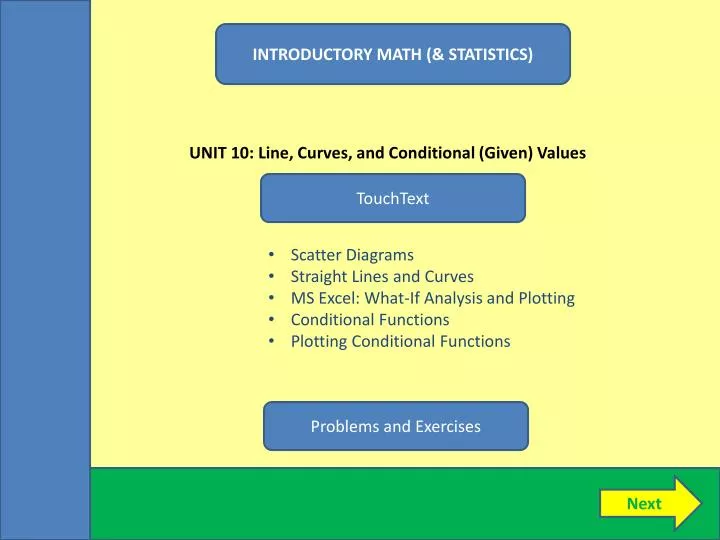
INTRODUCTORY MATH (& STATISTICS). UNIT 10: Line, Curves, and Conditional (Given) Values. TouchText. Scatter Diagrams Straight Lines and Curves MS Excel: What-If Analysis and Plotting Conditional Functions Plotting Conditional Functions. Problems and Exercises. Next.

E N D
INTRODUCTORY MATH (& STATISTICS) UNIT 10: Line, Curves, and Conditional (Given) Values TouchText • Scatter Diagrams • Straight Lines and Curves • MS Excel: What-If Analysis and Plotting • Conditional Functions • Plotting Conditional Functions Problems and Exercises Next
Graphing Two Variables We are interested in the relationship between two or more variables. When there are only two variables and one is a functionof the other (Y as a function of X, say), we can plot the relationship in X,Y space. Normally, the independentvariable (X) is on the horizontal axis, and the dependentvariable(Y) is on the vertical axis. Dictionary Take Notes Back Next
Linear Relationships Between X and Y A straight line connecting any two points has no curvature. Its slope is constant. If the relationship between X and Y is linear, then the relationship can be graphed in X,Y space as a straight line. The relationship can be written of the form: Dictionary Y = mX + b Slope Y-intercept This equation can be re-arranged in any mathematically acceptable way, but if it can be written in this form, then the coefficient in front of X (called “m” here) is the slope of the line in X,Y space, and the constant term (here, “b”) is the Y–intercept. Take Notes Back Next
Example of a Line Line example: Y = 10 + 2X Y-intercept = 10, slope = 2. Dictionary Take Notes Back Next
Linear Relationships: Negative Slope Line example #2: X + 2Y = 12. *This can be re-written as Y = 6 – 0.5X. Dictionary Y-intercept = 6; slope = - 0.5. Take Notes Back Next
Linear Relationships: Another Indicator Another way of determining whether or not the relationship between X and Y is a straight line, is to look at the exponent on the X variable. If the X-exponent equals one (i.e. not displayed), then the relationship is linear. Dictionary Y = 10 + 2X equivalent to Y = 10 + 2X1 Take Notes Back Next
Non-Linear Relationships: Using the X XxponentAs An Indicator When there is an exponent (other than 1) on the X variable, then the relationship will be non-linear (i.e. a curve). Dictionary • If the exponent k > 1 then the curve will get increasinglysteep – either upward or downward – from left to right. • If the exponent k < 1 then the curve will get decreasinglysteep, i.e. flatter, from left to right. Take Notes Back Next
Example: Curve, Positive Slope, Increasingly Steep If the exponent on X is greater than one, the relationship will be a curve sloping increasingly upward or increasingly downward. Dictionary Take Notes Back Next
Example: Curve, Negative Slope, Increasingly Steep If the exponent on X is greater than one, the relationship will be a curve sloping increasingly upward or increasingly downward. Dictionary Take Notes Back Next
Example: Curve, Positive Slope, Flatter If the coefficient on X is positive and the exponent on X is less than one, the relationship will be an upward-sloping curve getting flatter from left to right. Dictionary Y = -4 + 2X0.4 Take Notes Back Next
Example: Curve, Negative Slope, Flatter If the coefficient on X is negative and the exponent on X is less than one, the relationship will be a downward-sloping curve that gets flatter from left to right. Dictionary Y = 15 - 2X0.5 Take Notes Back Next
Exercises: Equations and Plotting The spreadsheet link below opens an MS Excel spreadsheet with instructions on how to enter and plot formulas. Follow the link; and practice entering and plotting formulas. To perform well in these exercises, students should be able to anticipate what the plot will look like before actually creating it, based upon the function that it is plotting. Dictionary Take Notes Back
Equations With More Than One Independent Variable Mathematically, everything learned thus far generalizes to equations with more than one independent variable. Dictionary Example: Y = 312 + 0.75X1 + 0.5X2 - 14.40X31.5X42. In this example, the dependent variable Y is a function of four independent variable: X1, X2, X3 and X4. As notation, the functional relationship would be written as: Y = f(X1, X2, X3, X4). Simply insert values for the for independent variables and solve for the dependent variable Y as before. Take Notes Back Next
Conditional Equations With More Than One Independent Variable As an analytical matter, one often wants to focus on the effects of only one independent variable at a time. This is imperative if one wishes to graph a relationship (on a flat, two dimensional space). Dictionary The solution is to fix the other independent variables at some amount(s), and then make the two-variable relationship under analysis a conditional relationship. Conditional functions are written with a “|” vertical bar inserted into the functional notation, to indicate that variables to the right of the bar are held at conditional values. Example: Y = f(X2|X1,X3,X4) Read: Y as a function of X2conditional on, or “given”, values for X1, X3 and X4. Take Notes Back Next
Conditional Function: Example Consider a demand curve (from economics class) of the form: QD = 120 – 3.5P + 0.1Y + 0.25PZ Where Dictionary P is the product’s own price Y is income PZ is a competing product’s price. Normally, only the demand curve (QD = f(P)) is graphed. But here, we make the entire demand function explicit and conditional: QD = f( P | Y, PZ) Take Notes Back Next
Conditional Function: Exercise The following Excel link is to a spreadsheet that again, asks the student to enter and plot formulas. This time, however, the formula involves three independent variables., and the plot is conditional on the values of the two “given” variables. Dictionary * The example is from a demand curve of the kind a student would get in an introductory economics class. The practice of drawing an inverse demand curve (P = f-1(Q)) instead of a standard demand function (Q = f(P)) creates problems that are addressed in this exercise. Take Notes Back
End of Unit 10 Questions and Problems There are no additional problems created for this Unit. Students are urged to practice working on the mathematics of functions and conditional functions; and on using the mathematical tools provided in MS Excel, on their own. Dictionary Take Notes Back End