Download
1 / 24
250 likes | 256 Views
Parameter Estimation: Maximum Likelihood Estimation Chapter 3 (Duda et al.) – Sections 3.1-3.2. CS479/679 Pattern Recognition Dr. George Bebis. Parameter Estimation. Bayesian Decision Theory allows us to design an optimal classifier using the Bayes rule:

E N D
Parameter Estimation:Maximum Likelihood EstimationChapter 3 (Duda et al.) – Sections 3.1-3.2 CS479/679 Pattern RecognitionDr. George Bebis
Parameter Estimation • Bayesian Decision Theory allows us to design an optimal classifier using the Bayes rule: • Estimating P(i) is usually not very difficult. • Estimating p(x/i) could be challenging: • Dimensionality of feature space is large. • Number of samples is often too small.
Parameter Estimation (cont’d) • Assumptions • A set of training samples D ={x1, x2, ...., xn} is provided where the samples were drawn according to p(x|wj). • p(x|wj) has some known parametric form: • Parameter estimation problem e.g., p(x /j) ~ N(μ, ) also denoted as p(x/j,q) or p(x/q)where q=(μ, Σ) Given D, find the best possible q
Problem Formulation • Consider cclasses and c training data sets (i.e., one for each class): • Given D1, D2, ...,Dc and a model p(x/ωj) ~ p(x/qj), for each class ωj , j=1,2,…,c, estimate: • If the samples in Dj provide no information about qi( ), we need to solve cindependent problems (i.e., one for each class). • D1, D2, ...,Dc q1, q2,…, qc
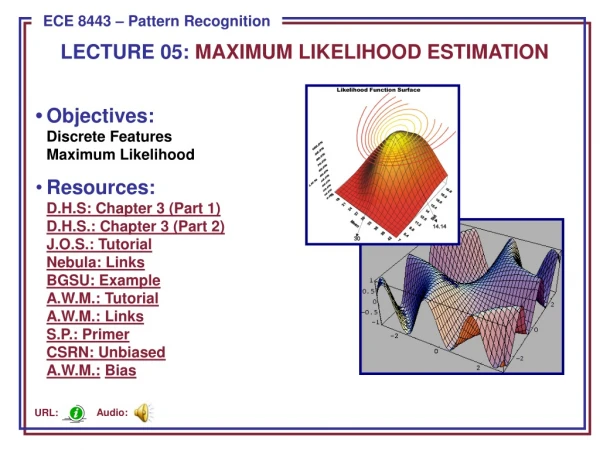
Main Methods • Maximum Likelihood (ML) • Views the parameters q as quantities whose values are fixed but unknown. • Estimates by maximizing the likelihood of obtaining the samples observed. • Bayesian Estimation (BE) • Views the parameters q as random variables having some known prior distribution p(q). • Observing new samples D, converts the prior p(q) to a posterior density p(q/ D) (i.e., the samples D revise our estimate of the distribution over the parameters).
ML Estimation - Solution • The ML estimate for D={x1,x2,..,xn} is the value that maximizesthe likelihood p(D/q): • This corresponds to the intuitive idea of choosing the value of 𝜃 that is most likely to give rise to the data. • Assuming that samples in D are drawn independently according to p(x/ωj):
ML Estimation - Solution (cont’d) • How can we find the maximum of p(D/ q) ? where (gradient)
ML Estimation Using Log-Likelihood • First, take the log for simplicity: • Need to maximizeln p(D/ θ): log-likelihood
Example red dots (training data) Assume unknown mean, known variance θ=μ
ML for Multivariate Gaussian Density:Case of Unknownθ=μ Assume Compute the gradient =
ML for MultivariateGaussian Density:Case of Unknown θ=μ(cont’d) • Set : • The solution is given by The ML estimate is simply the “sample mean”.
ML for Univariate Gaussian Density:Case of Unknown θ=(μ,σ2) • Assume • Compute the gradient θ =(θ1,θ2)=(μ,σ2) =
ML for Univariate Gaussian Density:Case of Unknown θ=(μ,σ2) (cont’d) p(xk/θ) p(xk/θ) p(xk/θ)
ML for Univariate Gaussian Density:Case of Unknown θ=(μ,σ2) (cont’d) =0 • Set =0 =0 • The solutions are given by: sample mean sample variance
ML for Multivariate Gaussian Density:Case of Unknown θ=(μ,Σ) • In the general case (i.e., multivariate Gaussian) the solutions are: sample mean sample covariance
Generalize ML Estimation:Maximum A-Posteriori Estimator (MAP) • Sometimes, we have some knowledge about θ. • Assume that θfollows some distribution p(θ). • MAP maximizes p(D/θ)p(θ) or ln [p(D/ θ)p(θ)]:
Maximum A-Posteriori Estimator (MAP) (cont’d) • What happens when p(θ) is uniform? MAP becomes equivalent to ML (i.e., ML is a special case of MAP!)
MAP for MultivariateGaussian Density:Case of Unknown θ=μ • Assume • Computeln [p(D/ μ)p(μ)]: • Maximizeln [p(D/ μ)p(μ)]: and (both are known)
MAP for MultivariateGaussian Density:Case of Unknown θ=μ(cont’d) • If , then • What happens when
Bias and Variance • How good are the ML estimates? • Two measures of “goodness” are used for statistical estimates • Bias:how close is the estimate to the true value? • Variance:how much does it change for different datasets?
Bias and Variance • The bias-variance tradeoff: in most cases, you can only decrease one of them at the expense of the other
Biased and Unbiased Estimates • An estimate is unbiased when • The ML estimate is unbiased, i.e., • The ML estimates and are biased:
Biased and Unbiased Estimates (cont’d) • How bad is this bias? - The bias is only noticeable when n is small. • The following are unbiased estimates of and
Comments • ML estimation is simpler than alternative methods. • ML provides more accurate estimates as the number of training samples increases. • If the assumptions about the model p(x/ θ) and independence of the samples are true, then ML works well.