Download
1 / 28
280 likes | 372 Views
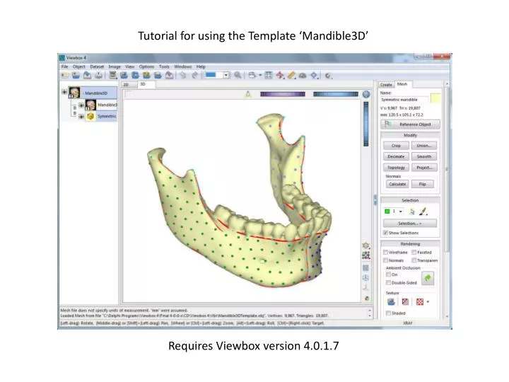
Tutorial for using the Template ‘Mandible3D’. Requires Viewbox version 4.0.1.7. Fixed landmarks: lateral and medial poles of the condyles coronoid tip infradentale linguale. Curves: Coronoid notch: between condyle and coronoid tip

E N D
Tutorial for using the Template ‘Mandible3D’ Requires Viewbox version 4.0.1.7
Fixed landmarks: • lateral and medial poles of the condyles • coronoid tip • infradentale • linguale • Curves: • Coronoid notch: between condyle and coronoid tip • Ramus: from coronoid tip down along external oblique line • External alveolar and internal alveolar: along the alveolar border, from the incisors to the most distally erupted molar • Symphysis: from Infradentale to Linguale • Lower border: from the posterior of the condyle, along the posterior border of the ramus and the inferior border of the mandibular body • Sliding landmarks on curves and on the surface: • 27 sliding landmarks on curves on each mandibular side • 11 sliding landmarks on the Symphysis curve • 80 surface sliding semilandmarks on each of the lateral sides • 60 surface sliding semilandmarks on each of the medial sides • Helper points: • 1 point at the approximate position of Gnathion
Start a New Patient and create a new Dataset using the Mandible3D Template:
Click on Mesh and then load the mesh from your hard disk: Select the Digitiser tool: Note: if the mesh icon does not have a flag next to it, then click the Reference Object button.
Notes Digitization of a new mandible begins by placing points: • Left Lateral Condyle • Left Medial Condyle • Left Coronoid • Right Lateral Condyle • Right Medial Condyle • Right Coronoid You do not need to place any of these points precisely. Just click (right-click) at their very approximate positions.
After placing the first 6 points. Notice that they were placed very approximately: To relocate the condyle points so that they lie on the poles of the condyles, open the drop-down menu and select “Relocate Points on Surface” (the coronoid points will be relocated later).
After relocating the condyle points: (of course you can adjust them later) The condyle points were moved by sliding them on the surface, as if the medial and lateral points repelled one another. In this way they eventually position themselves as far as possible to each other, i.e. on the poles of the condyles. The coronoid points will be relocated later.
Notes The next point, the helper point (Gnathion helper), is only used to facilitate placement of the curves by Viewbox. It is not used in any measurements or shape analyses. You do not need to position it precisely, just place it at any location on the symphysis, approximately where you would place Gnathion. After placing ‘Gnathion helper’ we need to set the curves on the surface of the mandible. The first curve is the left lower border. It should appear at approximately the correct position. Turn the mandible around so that you view it from the left side.
The mandible from the left side. The curve (in yellow) is approximately correct. Position the mouse on the Move icon and drag, so that the curve moves away from the mandible, in the direction of the thick arrow.
After moving the curve away from the mandible: Click the Project button. The curve will snap on the mandible. Each point of the curve (it has 18 adjustment points) will be projected on the closest point on the mandibular surface. Because the curve was positioned towards the lower right, the closest points will most likely be points on the lower and posterior border of the mandible, therefore very little, if any, adjustment will be needed.
After ‘projecting’ the curve on the mandible: You can adjust each of the points on the curve by moving them with the mouse. Place the mouse on the point: the mouse cursor changes into a thin double-arrow, then drag the point. When dragging, the point stays on the surface. Make sure that the curve starts just posterior to the condyle and ends at the midline. You can increase or decrease the number of points (if you do, it is a good idea to ‘project’ again).
Click the Auto All button and the curve semi-landmarks will be automatically located: The semi-landmarks are placed at predefined positions along the curve (these are not their final positions because later we will have them slide in order to minimize the bending energy). Click the Next button to move to the next curve (R Border). Digitise the right border in the same way and click the Auto All button again.
Both borders have been digitised: Use the drop-down menu to relocate the points again. This time, the coronoid points will move. They are ‘repelled’ by the points on the lower border and move towards the highest point on the coronoidprocess. ‘Relocate’ moves all points, so, instead of doing two relocations (one for the condylar points and one for the coronoid points), we could do only the one at this stage.
After relocating the coronoid points: Relocation is just a way to speed-up the process of digitising. It is not necessary and one could place the points just by inspection. Click the Next button to move on to the other curves. These are placed in a similar way. It is recommended to use ‘Auto All’ after placing each curve.
Notes • Use the trick of dragging the curve away from the surface and then projecting, so that the curve projects on the most prominent ridge. • If the points of the curve bundle up, then change the number of points. This re-distributes the points evenly along the curve. • Increase the number of points to allow the curve to approximate the surface better. Decrease the number of points to facilitate gross adjustments of the curve. Always ‘project’ after changing the number of points, to make sure that all points lie on the surface. • The points on the curves are not landmarks; they are for adjusting the shape of the curve only. It makes no difference how many there are; you can have different number of curve points for each patient. • Make sure that the curve does not project on the interior of the surface. Make the Mesh transparent to see if the curve is buried inside the surface. • Use Auto All after adjusting each curve. This places the landmarks on the curve and allows Viewbox to guestimate the best position for the next curve better.
All curves have been digitised: Now we need to digitise the surface semi-landmarks. These have been placed on the Template, so we will transfer them from the Template to this mandible. Since we have already digitised the curve semi-landmarks and the fixed landmarks, we can use them as guides. From the drop-down menu, select “Digitise Points based on TPS Warping of Template”
The surface points after transferring: Most of the surface points are not on the surface, so we open up the drop-down menu again and select “Project Points on Surface” (this may be slow).
The surface points after projecting: With a bit of luck, all points will be properly placed. However, some points may have been projected on the wrong side, so we need to check and correct them: Click on Finish to close the Digitisebox. Set mesh rendering to Transparent, then select the Dataset, instead of the mesh, in the Icon Area.
Prepare for checking points: Select <none> from the Views listbox. Click on the Select tool to select it. Right-click on the Select tool again and select “Select Area…” from the popup menu...
The Select Area window will open. This has two panels. The panel on the right contains all the points. The panel on the left has pre-defined ‘areas’, i.e. collections of points for easier selecting. Select the ‘Left lateral points area’ and click OK.
The points on the left lateral surface of the mandible are now selected: Notice that one point is inside the mandible. We can see it because the mesh is transparent. Position the mouse on the point; the mouse cursor changes to a double arrow. Drag the point slightly (all other points will temporarily disappear) and it will snap from the inside to the outside surface. Do the same for any other points that may be inside the surface.
Repeat for the other 3 ‘areas’: Right-click on the Select tool again and select “Select Area…” from the popup menu. Select each of the other ‘Areas’ and repeat the process until all points are now lying on the exterior surface of the mandible. When finished, click on the Select tool to de-activate it, then right-click on it, and select ‘Select None’ from the popup menu. Make all points visible again by selecting <all> in Views.
The finished result: All points and curves digitised. The mesh has been rendered in normal mode again. Save the Patient!
Notes • Mandibular meshes that have been created from CBCT scans may contain surfaces inside the mandible (roots of teeth, interior surface of the cortical bone, etc). These interior surfaces are a problem because a) they make Viewbox’s response slower, as they may consist of a large number of triangles, and b) landmarks may be projected on them instead of on the exterior surface. It is a good idea to delete such surfaces from the beginning. An easy way to do this is as follows:
The original mesh (from a medical CT): First make sure that the Normals have been properly computed: Click on Normals. Then click the Flip Normals button. Compare the two renderings. Choose the one in which the mandible seems most ‘fuzzy’ (see next slide).
Normals NOT correct Normals correct
Once the normals are correct, turn them off and render the mesh as transparent. Observe the inner surface in the image above. From the Selection menu, select “Select Non-Visible”. This procedure is slow. When done you should see that the inner surface has been selected (next slide).
Now delete the selected surface using the “Delete Selection” command.