Download
1 / 57
570 likes | 701 Views
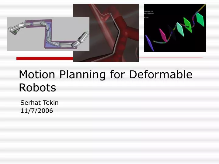
Motion Planning for Deformable Robots. Serhat Tekin 11/7/2006. Motivation. Motion planning is a classical problem Mostly for rigid or articulated robots Deformable variants are recent Massive configuration space even for simple cases Existing methods not directly applicable. Motivation.

E N D
Motion Planning for Deformable Robots Serhat Tekin 11/7/2006
Motivation • Motion planning is a classical problem • Mostly for rigid or articulated robots • Deformable variants are recent • Massive configuration space even for simple cases • Existing methods not directly applicable
Motivation • Why need deformable robots? • Applications in • Industry • CAD and virtual prototyping • Computer generated animation • Bioinformatics • Computer-aided surgery
Outline • Different approaches • Physically-based • Anshelevich et al. Rice University • Geometry-based • Bayazit et al. Texas A&M University • Constraint-based • Gayle et al. UNC at Chapel Hill • Conclusion
Outline • Different approaches • Physically-based • Anshelevich et al. Rice University • Geometry-based • Bayazit et al. Texas A&M University • Constraint-based • Gayle et al. UNC at Chapel Hill • Conclusion
Physically-based Approach • Builds upon a similar framework introduced for elastic plates • Lamiraux et al. Rice University • An extension to PRM that takes deformation energy into account • Volume deformations represented by a mass-spring lattice
Continuous Mechanical Model • Uses the linear elastic physical model • For a point v, energy density is defined by • F is the matrix of partial derivatives of the deformation functionγevaluated at γ-1(v) • The energy of γis
Discrete Spring Model • Approximates the continuous model • Two types of springs between the masses • Straight springs • Angular springs • Constant is picked according to type • Discritized energy function
Volume Deformation • Things to consider • Grasp/Manipulation constraints on volume • Restricts positions on some parts of the volume • i.e. fix the positions of some point masses • Energy minimization
Path Planning • Uses PRM for path planning • Local planner • Interpolates between manipulation constraints to form a sequence of intermediate constraints • Elasticity limits • Constants to prevent unnatural deformations • Plane strain limit: How much the material stretches locally • Curvature limit: How much the material bends locally
Results (on an SGI R10000) Deformable cable with fixed end (32x3x3 lattice)14.5 mins (average) Elastic pipe through a cube withan L-shaped hole (21x3x3 lattice)8h 39mins
Outline • Different approaches • Physically-based • Anshelevich et al. Rice University • Geometry-based • Bayazit et al. Texas A&M University • Constraint-based • Gayle et al. UNC at Chapel Hill • Conclusion
Geometry-based Approach • PRM extension, similar to the first method • Deformations are not represented by physical means • Aims at a reasonable-time limit with plausible deformations, rather than physical correctness
Overview • Critical steps in the algorithm • Roadmap construction • Querying and deformation
Roadmap Construction • Need to estimate the edge weights • Two different heuristics • Shrinkable robots • Use rigid robots with different scales • Edge weight is the sum of “shrink factor”s of endpoints • Allowing penetration • Work in C-space to estimate penetration depth • Sample n different C-space vectors(empirically, n = 20) • If any sample is collision free, accept • Minimum depth is used for the edge weight
Roadmap Construction • Shrinkable robot • Penetration • Swept volume of the path found
Query • Deformable robot used in the query phase • Collisions must be avoided by deformations • Configuration accepted if deformation energy below threshold • Edges with higher weights are likely to fail, so test them first
Deformations • Bounding-box deformation • Deformer pushes object into collision-free condition • ChainMail deformation • Similar to FFD • Deforming boundary box vertex affects neighbors • Free-form deformation (FFD) • Only used for visualization • Geometric deformation • Deform the colliding portion directly • Translate along surface normals
Deformations Geometric deformation: a) Colliding configuration b) Intersecting polygonsc) Deformed version Bounding-box deformation
Results (for “narrow” scenario)
Summary • Both methods are PRM extensions • Differ in the way they handle roadmaps and deformations • Physically-based • Deformation taken into account during roadmap construction • Deformations are physical simulations • Geometry-based • Robot treated as rigid during roadmap construction • Deformations are geometric
Advantages/Disadvantages • (+) Both methods offer a generalized framework to the problem • Same deformation scheme can be used with a different randomized planner • (-) Can handle only simple robots and environments • First approach is computationally expensive • Second one is not physically accurate
Outline • Different approaches • Physically-based • Anshelevich et al. Rice University • Geometry-based • Bayazit et al. Texas A&M University • Constraint-based • Gayle et al. UNC at Chapel Hill • Conclusion
Constraint-Based Motion Planning • M. Garber and M. Lin, Constraint-based motion planning using Voronoi diagrams. Proc. Fifth International Workshop on Algorithmic Foundations of Robotics (WAFR), 2002 • Reformulate the planning problem as a boundary value problem (BVP) • Builds on similarity between BVP and Motion planning • Map initial and goal configuration to boundary values • Map motion into a constrained dynamics function • Solvable through dynamical simulation
CBMP Goal • To find a (near) minimal set of constraints which are sufficient to solve the problem • Example: A 2D rigid robot in a simple environment • The robot must: • Reach a goal • Avoid obstacles
Constraints • Hints at how the object should move • Hard constraints: Must be satisfied at each step • No penetration or intersection with obstacles • Robot must stay within boundaries • Articulated links must stay together • Joint limits must be satisfied • Soft constraints: Encourage a certain behavior • Robot should follow a guiding path • Robot should move towards the goal configuration • Robot should avoid nearest obstacles
CBMP for Deformable Robots • DPlan: Builds upon CBMP • Represent deformation as a list of constraints • Represent energy minimization as a constraint • Two stage approach • Off-line roadmap generation • Simple PRM for a point robot • Possibly contains collisions • Runtime path query by constrained dynamic simulation • Performs deformation and local adjustments to path
Simulating Deformation • Represent deformation as a list of constraints • Considerations • Continuum representation • Energy minimization • Volume preservation • Interaction with the environment
Continuum Representation • Uses a simple Mass-Spring framework • Computationally inexpensive • Simple implementation and relatively easy interaction with the environment
Energy Minimization • Robot energy function (defined by springs): • k is spring constant, d is current distance, L is rest length • Relax the case, i.e. allow small changes to the volume
Volume Preservation • Relaxation • Measures internal pressure variations • Computes a pressure constraint force to adapt to changes in pressure • Uses a simplified model based on the Ideal Gas Law Force due to pressure on a surface Ideal Gas Law
Adjusting Pressure • Internal pressure constant defines the robot behavior • The RHS constant of Ideal Gas Law (nRgT) is assigned by trial-and-error Low Pressure Medium Pressure High Pressure
Interaction • Hard constraints for interaction with environment • Bounding-volume collision detection • Assumes collision if robot is within a tolerance to an obstacle • Applies impulses and repulsion forces at the affected masses • Soft constraints for global behavior • Path following
Deformation Step • Perform collision detection • Handle collisions to enforce non-penetration constraints • Accumulate spring forces Fs • Compute the volume V of the object • Set P = nRgT / V • For each face f on the geometry • Set Fp = PA • For each vertex v of f • Find the pressure forces on v by adding Fpdivided by the number of faces incidental to v
Summary • Builds upon CBMP • Adds constraints for deformation, path following, and interaction with the environment • Uses a simplified global path to help escape local minima while using CBMP to make local adjustments to ensure a collision-free path
Advantages • Allows for complex robots • Computes physically-plausible deformations • Performs sampling in low-degree of freedom space (i.e. workspace)
Limitations • Does not ensure a path will be found • Cannot guarantee accurate deformations • Restricted ability to represent robots with sharp edges • Applicable only to closed robots • Limited scalability
Results • Ball in cup • Many spheres Cup - 500 Polygons Robot – 320 Polygons Spheres - 3200 Polygons Robot – 320 Polygons
Results • Walls with holes Walls - 216 Polygons per wall Robot – 720 Polygons
Results • Tunnel Tunnel - 72 Polygons Robot – 720 Polygons
Improving Performance • Support for complex environments • FlexiPlan: Path Planning for Deformable Robots in Complex Environments (FlexiPlan) • Builds upon DPlan by improving primary bottlenecks • Guiding path improvements • Simulation improvements
Improvements • More optimal global guiding path • Samples along the medial axis of the workspace to create a path (Medial Axis PRM) • Generalized Voronoi Diagram is another possibility • Computed efficiently with GPUs • Simulation improvements • Mass-Spring simulation • More stable (Semi-Implicit Verlet integration) • Supports angular springs to counteract shearing • Better collision detection scheme
Collision Detection • Dominating factor in running time • DPlan only uses a bounding volume to remove unnecessary checks • BVH is not a viable option • Robot is often too close to obstacles in most scenarios • BVH would not eliminate most tests and incur an update cost • Speed up collision tests by • 2.5D overlap test • Set-based computation
2.5D Overlap Test • Based on CULLIDE • Choose a viewing direction • Check whether R is fully visible with respect to O along that direction • Utilize GPU occlusion query
Reliable GPU Check • Might miss overlaps due to pixel precision • To prevent this • Determine the size of a pixel • Compute Minkowski sum of the obstacles and robot with a pixel • Conservative, since may include pixels from geometry which does not overlap
Set-Based Computation • Maintains a PCS (Potentially Colliding Set) throughout computation • Initially everything is in the PCS • Uses overlap tests to remove obstacles from the PCS • Do exact collision detection on the PCS • If number of primitives is small, test all pariwise combinations • Else, use bounding boxes for speed-up