CS 188: Artificial Intelligence Spring 2007

1. CS 188: Artificial IntelligenceSpring 2007 Lecture 12: Graphical Models 2/22/2007 Srini Narayanan – ICSI and UC Berkeley

2. Probabilistic Models • A probabilistic model is a joint distribution over a set of variables • Given a joint distribution, we can reason about unobserved variables given observations (evidence) • General form of a query: • This kind of posterior distribution is also called the belief function of an agent which uses this model Stuff you care about Stuff you already know

3. Independence • Two variables are independent if: • This says that their joint distribution factors into a product two simpler distributions • Independence is a modeling assumption • Empirical joint distributions: at best “close” to independent • What could we assume for {Weather, Traffic, Cavity, Toothache}? • How many parameters in the joint model? • How many parameters in the independent model? • Independence is like something from CSPs: what?

4. Example: Independence • N fair, independent coin flips:

5. Example: Independence? • Most joint distributions are not independent • Most are poorly modeled as independent

6. Conditional Independence • P(Toothache,Cavity,Catch)? • If I have a cavity, the probability that the probe catches in it doesn't depend on whether I have a toothache: • P(catch | toothache, cavity) = P(catch | cavity) • The same independence holds if I don’t have a cavity: • P(catch | toothache, cavity) = P(catch| cavity) • Catch is conditionally independent of Toothache given Cavity: • P(Catch | Toothache, Cavity) = P(Catch | Cavity) • Equivalent statements: • P(Toothache | Catch , Cavity) = P(Toothache | Cavity) • P(Toothache, Catch | Cavity) = P(Toothache | Cavity) P(Catch | Cavity)

7. Conditional Independence • Unconditional (absolute) independence is very rare (why?) • Conditional independence is our most basic and robust form of knowledge about uncertain environments: • What about this domain: • Traffic • Umbrella • Raining • What about fire, smoke, alarm?

8. The Chain Rule II • Can always factor any joint distribution as an incremental product of conditional distributions • Why? • This actually claims nothing… • What are the sizes of the tables we supply?

9. The Chain Rule III • Trivial decomposition: • With conditional independence: • Conditional independence is our most basic and robust form of knowledge about uncertain environments • Graphical models help us manage independence

10. The Chain Rule IV • Write out full joint distribution using chain rule: • P(Toothache, Catch, Cavity) = P(Toothache | Catch, Cavity) P(Catch, Cavity) = P(Toothache | Catch, Cavity) P(Catch | Cavity) P(Cavity) = P(Toothache | Cavity) P(Catch | Cavity) P(Cavity) Cav P(Cavity) • Graphical model notation: • Each variable is a node • The parents of a node are the other variables which the decomposed joint conditions on • MUCH more on this to come! T Cat P(Toothache | Cavity) P(Catch | Cavity)

11. Combining Evidence P(cavity | toothache, catch) =  P(toothache, catch | cavity) P(cavity) =  P(toothache | cavity) P(catch | cavity) P(cavity) • This is an example of a naive Bayes model: C E1 E2 En

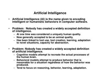
12. Graphical Models • Models are descriptions of how (a portion of) the world works • Models are always simplifications • May not account for every variable • May not account for all interactions between variables • What do we do with probabilistic models? • We (or our agents) need to reason about unknown variables, given evidence • Example: explanation (diagnostic reasoning) • Example: prediction (causal reasoning) • Example: value of information

13. Bayes’ Nets: Big Picture • Two problems with using full joint distributions for probabilistic models: • Unless there are only a few variables, the joint is WAY too big to represent explicitly • Hard to estimate anything empirically about more than a few variables at a time • Bayes’ nets (more properly called graphical models)are a technique for describing complex joint distributions (models) using a bunch of simple, local distributions • We describe how variables locally interact • Local interactions chain together to give global, indirect interactions

14. Graphical Model Notation • Nodes: variables (with domains) • Can be assigned (observed) or unassigned (unobserved) • Arcs: interactions • Similar to CSP constraints • Indicate “direct influence” between variables • For now: imagine that arrows mean causation

15. Example: Coin Flips • N independent coin flips • No interactions between variables: absolute independence X1 X2 Xn

16. Example: Traffic • Variables: • R: It rains • T: There is traffic • Model 1: independence • Model 2: rain causes traffic • Why is an agent using model 2 better? R T

17. Example: Traffic II • Let’s build a causal graphical model • Variables • T: Traffic • R: It rains • L: Low pressure • D: Roof drips • B: Ballgame • C: Cavity

18. Example: Alarm Network • Variables • B: Burglary • A: Alarm goes off • M: Mary calls • J: John calls • E: Earthquake!

19. Bayes’ Net Semantics • Let’s formalize the semantics of a Bayes’ net • A set of nodes, one per variable X • A directed, acyclic graph • A conditional distribution for each node • A distribution over X, for each combination of parents’ values • CPT: conditional probability table • Description of a noisy “causal” process A1 An X A Bayes net = Topology (graph) + Local Conditional Probabilities

20. Probabilities in BNs • Bayes’ nets implicitly encode joint distributions • As a product of local conditional distributions • To see what probability a BN gives to a full assignment, multiply all the relevant conditionals together: • Example: • This lets us reconstruct any entry of the full joint • Not every BN can represent every full joint • The topology enforces certain conditional independencies

21. Example: Coin Flips X1 X2 Xn Only distributions whose variables are absolutely independent can be represented by a Bayes’ net with no arcs.

22. Example: Traffic R T

23. Example: Alarm Network

24. Example: Naïve Bayes • Imagine we have one cause y and several effects x: • This is a naïve Bayes model • We’ll use these for classification later

25. Example: Traffic II • Variables • T: Traffic • R: It rains • L: Low pressure • D: Roof drips • B: Ballgame L R B D T

26. Size of a Bayes’ Net • How big is a joint distribution over N Boolean variables? • How big is an N-node net if nodes have k parents? • Both give you the power to calculate • BNs: Huge space savings! • Also easier to elicit local CPTs • Also turns out to be faster to answer queries (next class)

27. Building the (Entire) Joint • We can take a Bayes’ net and build the full joint distribution it encodes • Typically, there’s no reason to build ALL of it • But it’s important to know you could! • To emphasize: every BN over a domain implicitly represents some joint distribution over that domain

28. Example: Traffic • Basic traffic net • Let’s multiply out the joint R T

29. Example: Reverse Traffic • Reverse causality? T R

30. Causality? • When Bayes’ nets reflect the true causal patterns: • Often simpler (nodes have fewer parents) • Often easier to think about • Often easier to elicit from experts • BNs need not actually be causal • Sometimes no causal net exists over the domain (especially if variables are missing) • E.g. consider the variables Traffic and Drips • End up with arrows that reflect correlation, not causation • What do the arrows really mean? • Topology may happen to encode causal structure • Topology really encodes conditional independencies

31. Creating Bayes’ Nets • So far, we talked about how any fixed Bayes’ net encodes a joint distribution • Next: how to represent a fixed distribution as a Bayes’ net • Key ingredient: conditional independence • The exercise we did in “causal” assembly of BNs was a kind of intuitive use of conditional independence • Now we have to formalize the process • After that: how to answer queries (inference)

32. Estimation • How to estimate the a distribution of a random variable X? • Maximum likelihood: • Collect observations from the world • For each value x, look at the empirical rate of that value: • This estimate is the one which maximizes the likelihood of the data • Elicitation: ask a human! • Harder than it sounds • E.g. what’s P(raining | cold)? • Usually need domain experts, and sophisticated ways of eliciting probabilities (e.g. betting games)

33. Estimation • Problems with maximum likelihood estimates: • If I flip a coin once, and it’s heads, what’s the estimate for P(heads)? • What if I flip it 50 times with 27 heads? • What if I flip 10M times with 8M heads? • Basic idea: • We have some prior expectation about parameters (here, the probability of heads) • Given little evidence, we should skew towards our prior • Given a lot of evidence, we should listen to the data • How can we accomplish this? Stay tuned!