Download
1 / 28
280 likes | 600 Views
Numerical Simulation of Infrasound Propagation, including Wind, Attenuation, Gravity and Non-linearity. Catherine de Groot-Hedlin Scripps Institution of Oceanography University of California, San Diego. Overview. Linear propagation Finite difference, time-domain method (FDTD) vs. rays

E N D
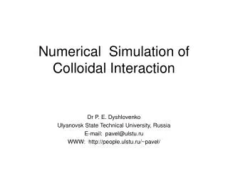
Numerical Simulation of Infrasound Propagation, including Wind, Attenuation, Gravity and Non-linearity Catherine de Groot-Hedlin Scripps Institution of Oceanography University of California, San Diego
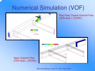
Overview • Linear propagation • Finite difference, time-domain method (FDTD) vs. rays • Examples: • Advected (windy) propagation into a shadow zone • Comparison of advected propagation with and without attenuation • Comparison of low frequency advected propagation with and without gravity • Nonlinear propagation (future work) • Use of mesh-free methods • Example: • solution of Berger’s equation
Pressure wavefields in a shadow zone • FDTD pressure solutions shows infrasound energy entering “shadow” zones
FDTD waveform results vs. rays • Shadow zone as indicated by rays • Low frequency infrasound is diffracted into the shadow zone
Finite-Difference, Time-Domain method Field variables are defined only at nodes, e.g. in a staggered grid Vx are leftward-pointing arrows Vz are upward-pointing arrows P nodes are at the center of cells • Equations are discretized, i.e. • Useful for modeling SMOOTH pressure fields, i.e. linear propagation
Attenuation Equations for propagation in a windy, absorptive medium • Equation for acoustic pressure • Equation for particle velocity • The viscosity is approximately constant (but attenuation is not)
Attenuation and Dispersion Combine equations (set wind=0) to get a 2nd order equation for pressure: and derive a solution of the type where gives the dispersion cp() and the attenuation
Dispersion • Predicted dispersion for a constant viscosity coefficient =1.7x10⁻⁵ kg m-1 s-1 • Dispersion is negligible below 120 km altitude
predicted attenuation solution for =1.7x10⁻⁵ kg m-1 s-1 Atmospheric attenuation
Environmental model • Source at 50 km • Source has peaks at f=0.01, 0.04, and 0.07 Hz
Ray results • Source at 50 km altitude • Receivers along ground at 50 km intervals from -300 km to 300 km • Arrivals on ground are direct arrivals (DA) and thermospheric refractions (TR) TR TR DA
Propagation with (top) and without (bottom) attenuation • T = 192 s
Propagation with (top) and without (bottom) attenuation • T = 384 s
Propagation with (top) and without (bottom) attenuation • T = 576 s
Propagation with (top) and without (bottom) attenuation • T = 768 s
Propagation with (top) and without (bottom) attenuation • T = 960 s shows attenuation of thermospheric refractions
Comparison of waveforms and spectra in attenuating vs. non-attenuating media attenuating media non-attenuating media Direct arrivals are minimally attenuated Thermospheric refractions are attenuated at 0.07 Hz, not at 0.01 Hz, for refractions at altitudes > 110 km.
Effect of Gravity on Infrasound • Infrasound propagtion equations, including gravity:
Low frequency source for infrasound propagation example, including gravity • Source consists of the superposition of 3 wavelets • Low frequency wavelet has energy at f<buoyancy frequency • Higher frequency wavelets should be minimally affected by inclusion of gravity terms
Propagation with (top) and without (bottom) gravity By T=640 s, low frequencies are strongly reflected from the sound speed gradient at 100km
Propagation with (top) and without (bottom) gravity T=1024 s
Propagation with (top) and without (bottom) gravity T=1408 s
Comparison of waveforms and spectra for low frequencies, with (left) and without (right) gravity terms Not including gravity terms Including gravity terms Large differences in pressure, particularly at low frequencies
Non-linear propagation • Steep gradients in the acoustic wave solution • Finite difference methods, or spectral methods would require a VERY high level of discretization • Instead, use a RADIAL BASIS FUNCTION method
Radial Basis Function method • The RBF method is meshfree • The grid is refined or coarsened depending on the level of accuracy needed • Solution is defined at all points, not just at nodes • Nonlinear propagation equations • pressure • Incompressible Navier-Stokes for particle velocity • The latter is related to Burgers equation
Conclusions • Have developed a working code to compute linear infrasound propagation through a windy atmosphere • Plan to run it to model propagation of WSMR shots to regional distances (where shock waves aren’t observed) • Am working on non-linear propagation code • Plan to run it to model propagation of WSMR shots to the near-field (where shock waves are observed) • Work on gravity waves in a windy environment is still a work in progress