Download
1 / 33
360 likes | 534 Views
Soil Solution Sampling Soluble Complexes Speciation Thermodynamic Stability Constant. Extraction Methods Collect drainage water in situ Reaction with collection vessel Must be at or near saturation High variability Displace with an immiscible liquid

E N D
Soil Solution Sampling Soluble Complexes Speciation Thermodynamic Stability Constant
Extraction Methods Collect drainage water in situ Reaction with collection vessel Must be at or near saturation High variability Displace with an immiscible liquid As by F3Cl3C2 in centrifuge (ρ = 1.58 g cm-3) Displace using air pressure (positive or vacuum) Reaction with filter Must be at or near saturation Displace using centrifugal force Generally, the extract cannot be identical to the true soil solution
Criticize this approach. Particle density = 2.62 g cm-3 and bulk density = 1.32 g cm-3 so that porosity = 0.50. What is the composition of saturated soil solution? Equilibrate 10 g water + 1 g soil, centrifuge and analyze 5 g water + 1 g soil 5 g water + 5 g soil 10 5 1 0.37 Empirically model Ca2+, Mg2+, …, SO42-, … and extrapolate.
Soluble Complexes Complex consists of a molecular unit (e.g., ion) as a center to which other units are attracted to form a close association Examples include Si(OH)4 and Al(OH)2+ with Si4+ and Al3+ as the central unit and OH- as ligands If two or more functional groups of a ligand are coordinated to a central metal, complex is called a chelate
If central unit and ligands are in direct contact, complex is inner-sphere If one or more H2O in between, complex is outer-sphere If ligands are H2Os, complex is solvation complex (e.g., Ca(H2O)62+) What would be orientation of H2Os? Mg2+(aq) + SO42-(aq) = MgSO4(aq) Given that –COO- tends to form water bridges to soil minerals via divalent cations adsorbed onto mineral surfaces, is the MgSO4 complex inner- or outer-sphere?
Kinetics of complex formation are fast Assume described by rate of disappearance of the metal as in the rate of its concentration decrease, -d[Mg2+] / dt = Rf – Rr where forward and reverse rates are affected by the temperature, pressure and composition of the solution Further, typically, -d[Mg2+] / dt = kf [Mg2+]α[SO42-]β – kr[MgSO4]γ αth order with respect to Mg2+
If tracked formation under conditions of excess SO42-, could determine α -d[A] / dt = kf [A]α 0th -d[A] / dt = kf and [A] = -kft + [Ao] 1st - d[A] / dt = kf[A] and ln[A] = -kft + ln[Ao] 2nd - d[A] / dt = kf[A]2 and 1/[A] = kft + 1/[Ao]
What if -d[Mg2+] / dt = kf [Mg2+][SO42-] – kr[MgSO4] at equilibrium 0 = kf [Mg2+][SO42-] – kr[MgSO4] [MgSO4] / [Mg2+][SO42-] = kf / kr = cKs Do problem 2.
Al3+ + F- = AlF2+ -d [Al3+] / dt = kf [Al3+][F-] – kr [AlF2+] At early stage of reaction, ignore reverse rate and since initial concentrations of Al3+ and F- are the same, [F-] = [Al3+], giving -d [Al3+] / dt = kf [Al3+]2 or -d [Al3+] / [Al3+]2 = kf dt which integrates to 1 / [Al3+] – 1 / [Al3+]0 = kf t Now what is the time when ½ of the Al3+ has reacted, i.e., the half life? 1 / ½ [Al3+]0 – 1/ [Al3+]0 = kf t½ or t½ = (1 / kf) (1 / [Al3+]0) = 909 s @ pH 3.9, given kf = 110 M-1 s-1 = 138 s @ pH 4.9, given kf = 726 M-1 s-1
Speciation Equilibria Assumption of fast complex formation and slow redox / precipitation Al speciation example Limit possible ligands to SO42-, F- and fulvic acid (L-) Set pH = 4.6 for which AlOH2+ is major hydroxide complex Ignore polymeric forms of aluminum [Al]T = [Al3+] + [AlOH2+] + [AlSO4+] + [AlF2+] + [AlL2+] Use conditional stability constants to express concentrations in terms of [Al3+], [OH-] or [H+] and concentrations of ligand species
[AlOH2+] = cK1 [Al3+][OH-] [AlSO4+] = cK2 [Al3+][SO42-] [AlF2+] = cK3 [Al3+][F-] [AlL2+] = cK4 [Al3+][L-] [Al]T = [Al3+] { 1 + cK1 [OH-] + cK2 [SO42-] + cK3 [F-] + cK4 [L-]}
Similarly, [SO42-]T = [SO42-] { 1 + cK2 [Al3+]} [F-]T = [F-] { 1 + cK3 [Al3+]} [L-]T = [L-] { 1 + cK4 [Al3+]}
Now proceed iteratively, Step 1 begin [Al3+] = [Al]T / { cK1 [OH-] + cK2 [SO42-] + cK3 [F-] + cK4 [L-]} where [OH-] is known from pH and concentration of other ligands are assumed equal to their known total concentration Concentrations of ligands other than OH- then calculated, as with [SO42-] = [SO42-]T / { 1 + cK2 [Al3+]} Step 1 end
Use revised concentrations of ligands to improve estimate of [Al3+], beginning Step 2 Continue until convergence reached Change in estimated concentrations from Stepi to Stepi + 1 < arbitrary criterion
Limitations to predicting speciation Completeness –may ignore important reactions (redox and speciation) Insufficient data –do not have conditional stability constants Analytical methodology –short-comings as in failure to distinguish between monomeric / polymeric or dissolved / particulate forms Assumption of equilibrium –ignores kinetics Field soils –conditions vary from those for which cKis determined; spatial / temporal variability, particularly mass inputs / outputs
Spreadsheet calculation problem [Al]T = 0.000010 M [SO42-]T = 0.000050 M [F-]T = 0.000002 [L-]T = 0.000010 pH = 4.60 cK1 = 109.00 M-1 cK2 = 103.20 cK3 = 107.00 cK4 = 108.60 Solve for all forms See spreadsheet. Also, do problem 6.
The distribution coefficients, αis, = [H2CO3] / [CO3T], etc., where [CO3T] = [H2CO3] + [HCO3-] + [CO32-] [1] Using the given CKSs, [HCO3-] = CK2 [H+] [CO3-2] but [CO32-] = [H2CO3] / (CK1 [H+]2) so [HCO3-] = (CK2 / CK1) ([H2CO3] / [H+]) and substituting in [1] gives [CO3T] = [H2CO3] {1 + (CK2 / CK1) / [H+] + 1 / (CK1 [H+]2)} and using [H+] = 10-pH the distribution coefficient for H2CO3 is αH2CO3 = 1 / {1 + 10-6.4 10pH + 10-16.7 102pH}
Proceeding similarly, αHCO3 = 1 / {106.4 10-pH + 1 + 10-10.3 10pH} αCO3 = 1 / {10-16.7 10-2pH + 1010.3 10-pH +1} Now, when is HCO3- dominant, i.e., αHCO3 ≥ 0.5? This is the case when {106.4 10-pH + 1 + 10-10.3 10pH} ≤ 2, no? This is almost the case when either pH = 6.4 or pH = 10.3 because at either pH, {106.4 10-pH + 1 + 10-10.3 10pH} is only slightly greater than 2, e.g., {106.4 10-6.4 + 1 + 10-10.3 106.4} = 1 + 1 + 0.00013 = 2.00013 Thus, HCO3 is (approximately) dominant at 6.4 ≤ pH ≤ 10.3
The earlier [Al3+] speciation problem can be handled more efficiently. Express the concentrations of ligands in terms of [Al3+] and total concentration of each ligand to give, [Al3+] = [Al]T / { (cK1 KW / [H+]) + (cK2 [SO42-]T / {1 + cK2 [Al3+]}) + (cK3 [F-]T / {1 + cK3 [Al3+]}) + (cK4 [L-]T / {1 + cK4 [Al3+]})} and approximate a solution for [Al3+] (below). In turn, the equilibrium concentrations of all species are known from the relations, [SO42-] = [SO42-]T / {1 + cK2 [Al3+]}, etc. Of course, there remains the problem that the various cKis may be unknown. This can be handled if the thermodynamic stability constants are known.
Note on Newton-Raphson Method [Al3+] = [Al]T / { (cK1 KW / [H+]) + (cK2 [SO42-]T / {1 + cK2 [Al3+]}) + (cK3 [F-]T / {1 + cK3 [Al3+]}) + (cK4 [L-]T / {1 + cK4 [Al3+]})} can be quickly approximated using this technique. As an example, solve the cubic, T = a1X +a2X2 + a3X3. First, write F(X) as F = a1X + a2X2 + a3X3 – T If guessed a value of X that gives F = 0, then T = a1X + a2X2 + a3X3 and no need to go further, but likely F 0. In this case, differentiate F(X) to give, dF / dX = a1 + 2a2X + 3a3X2 If the slope is evaluated at the initial guess, X1, an estimated solution, X2, is calculated from the definition of slope as rise / run, i.e., (0 – F1) / (X2 – X1) = dF / dX Repeat steps to estimate an arbitrarily accurate solution. Next figure illustrates.
guess second calculated X calculated X based on guess
Thermodynamic Stability Constant Activities instead of concentrations [MgSO4] / [Mg2+][SO42-] = cKs (MgSO4) / (Mg2+)(SO42-) = Ks but activity coefficients, i, convert from cKs to Ks, as with 2+ [Mg2+] = (Mg2+) So that if the ionic strength of the solution is known, the activity coefficients can be calculated and the appropriate conditional stability constant calculated as for this example, cKs = (2+ 2+ / 0) Ks
Debye-Hückel Notes on Chemical Potential Recall ΔG = ΔGo + RT ln K Chemical potential of i, μi, = (∂G / ∂ni)T,P , is related to activity of i, ai, by μi = μio + RT ln ai For the reaction aA + bB = cC + dD, (cμC + dμD – aμA – bμB) = (cμCo + dμDo – aμAo – bμBo) + RT ln (aAaaBb / aCcaDd) So, ΔG = (cμC + dμD – aμA – bμB) and ΔGo = (cμCo + dμDo – aμAo – bμBo). At equilibrium, ΔG = Σviμi, that is, using the above reaction, cμC + dμD = aμA + bμB
Development of Ion Activity Coefficient Write chemical potential in terms of concentration and activity coefficient, a = γm, and consider deviation from ideal behavior (γ < 1) is due to electrostatic interactions among ions, i.e., μ = μEL + μ* = RT ln γ + RT ln m, i.e., μEL = RT ln γ The idea is to relate μEL = RT ln γ to electric potential, φ*, in the vicinity of an ion. Take the single, central ion as a point charge for which the radial electric potential is (1 / r2) d (r2 (dφ / dr)) / dr = - 4πρ / D [2A] where ρ is charge density and D is dielectric constant. [2A], Poisson’s equation, arises in classical electromagnetic theory from relationships among charge density, electric field and electric potential. The electric field is given by the (-) potential gradient and the gradient of the electric field on the surface of a volume containing charge depends directly on the charge contained. So, charge can be expressed in terms of the (-) second derivative of potential. In this case, the equation is one-dimensional (radially symmetric).
To solve [2A] ρ must be expressed in terms of potential, φ. Since ρ = Σzieni, where zi is valance, e is single electronic charge and ni is concen- tration, ni can be related to potential by ni = nioexp(-zieφ /kT) [2B] where nio is average, bulk concentration (ions per mL) , k is the Boltzmann constant (R / NA) and T is absolute temperature. [2B] arises in statistical mechanics, so it is probabilistic. The notion is for a given total amount of energy in a system, the bodies (molecules, etc. ) that comprise the system are distributed among the essentially infinite number of energy microstates possible, but more commonly exist in lower energy states (-zieφ being energy). The exponential arises from a logrithmic approximation for factorials (probability calculations), and the denominator, kT (= RT / NA), comes from thermodynamic calculations.
(1 / r2) d (r2 (dφ / dr)) / dr = -(4π / D) Σzienioexp(-zieφ /kT) If the exponential is expressed as a series and truncated at the first two terms, 1 – zieφ / kT, (1 / r2) d (r2 (dφ / dr)) / dr = -(4π / D) Σzienio + (4π / D) Σzi2e2nioφ / kT Electrical neutrality results in the first term on the right hand side being zero, leaving (1 / r2) d (r2 (dφ / dr)) / dr = (4π / D) Σzi2e2nioφ / kT for which (4π / D) Σzi2e2nioφ / kT is written as κ2φ, i.e., κ2 = (4π / D) Σzi2e2nio / kT (1 / r2) d (r2 (dφ / dr)) / dr = κ2φ
The final matter is to relate potential, φ* = - (zieκ / D), to chemical potential, μEL (= RT ln γ). The approach taken is to charge a mole of central ions, each within the potential of its ion atmosphere, from zero to its actual charge, μEL = NA φ* d(zie) = NA-(zieκ / D) d(zie) = -NA zi2e2κ / 2D If κ = [(4π / D) Σzi2e2nio / kT]1/2 is substituted, μEL = -NA zi2e2 [(4π / D) Σzi2e2nio / kT]1/2 / 2D and from μEL = RT ln γ log γi = -NA zi2e2 [(4π / D) Σzi2e2nio / kT]1/2 / (2.303 2DRT)
Since the concentrations, nio, are in ions per mL and the final form of this model for a single ion activity coefficient is written in terms of ionic strength (I = ½ Σzi2mi, m is moles / kg), log γi = - zi2 [NA2e3 / (2.303 (DRT)3/2)][2πρ /1000]1/2 I1/2 where ρ is solution density. For water at 25 oC, the two bracketed factors multiply to 0.511, and log γi = -0.511 zi2 I1/2 Debye-Hückel limiting –applicable for I < 0.01
If consider ion is not a point charge, the earlier constant A (= zie / D) is expressed as, A = zie / D [ exp (κa) / (1 + κa)] where a is the minimum distance of approach. This leads to an expression for the potential due to the ion atmosphere about the central ion φ* = - zieκ / (D [1 + κa]) Integrating to find μEL, relating μEL to the activity coefficient (μEL = RT ln γ) and solving for γ gives log γ = -A Zi2 {I0.5 / [ 1 + BaiI0.5 ]} Applicable for I < 0.1
Models for ionic activity coefficients based on ionic strength, I where I = 0.5 Zk2 [m] Debye-Huckel Limiting Log i = -0.511 zi2 I1/2 Debye-Huckel log i = -A Zi2 {I0.5 / [ 1 + BaiI0.5 ]} Davies log i = -A Zi2 ( {I0.5 / [ 1 + I0.5]} – 0.3 I) where A = 0.512
Semiempirical models for uncharged species are log ML = -0.192 I / [ 0.0164 + I], for monvalent cations (M = Na+ etc.) log ML = -0.300 I, for divalent cations (M = Ca2+ etc.) log HL = 0.100 I, for proton complexes
A useful empirical relationship for soils is the Marion-Babcock model which relates ionic strength to electrical conductivity log I = 1.159 + 1.009 log where is electrical conductivity in dS m-1 Do problem 15 (next slide). Problems 4, 7 and 13
The equilibrium expressions in terms of CKS and KS are related by KS = (AlSO4+) / (Al3+)(SO42-) = CKS+ / 3+ 2- Thus, CKS / KS = 3+ 2- / + So since I increases with electrical conductivity, , through Marion-Babcock, whether CKS increases or decreases with increasing I, depends on the relative effect of increasing I on the ratio, 3+ 2- / +. Using the Debye-Hückel limiting, log γi = -0.511 zi2 I1/2, to illustrate, 3+ 2- / + = 10-0.511 (9 + 4 - 1) I½= 10-6.132I½