Download
1 / 42
420 likes | 545 Views
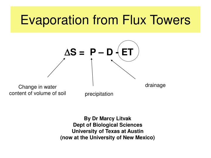
Evaporation from Flux Towers. S = P – D - ET. drainage. Change in water content of volume of soil. precipitation. By Dr Marcy Litvak Dept of Biological Sciences University of Texas at Austin (now at the University of New Mexico). Energy budgeting approach. Latent Heat flux.

E N D
Evaporation from Flux Towers S = P – D - ET drainage Change in water content of volume of soil precipitation By Dr Marcy Litvak Dept of Biological Sciences University of Texas at Austin (now at the University of New Mexico)
Energy budgeting approach Latent Heat flux How do you partition H and E?? Can directly measure each of these variables Sensible Heat flux
Net Ecosystem Production Eddy Covariance Directly measure how much CO2 or H2O vapor blows in or out of a site in wind gusts. Integrated measure of ecosystem fluxes Link changes in [CO2] or [H2O] in the air above a canopy with the upward or downward movement of that air
Flux CO2 = w ’ CO2’ Net Ecosystem Exchange 30 minute timescale Updraft [CO2] > downdraft [CO2] Flux >0 carbon source Updraft [CO2] < downdraft [CO2] Flux < 0 carbon sink
1000 Sunlight 800 600 Sunlight (Wm-2) • The net CO2 flux is calculated for each half hour from the measurements of vertical wind and CO2 concentration. • A positive flux indicates a net loss of CO2 from the surface (respiration) and a negative flux indicates the net uptake of CO2 (photosynthesis) 400 200 0 146.0 146.5 147.0 147.5 148.0 5 0 -5 CO2 Exchange (mmol m-2 s-1) -10 -15 CO2 Exchange -20 12 AM 12PM 12AM 12PM 12AM May 26, 2000 May 27, 2000
CO2 Exchange (mmol m-2 s-1) • A years worth of half-hour data can be summed to determine how much Carbon the ecosystem gained or lost 5 4 Annual C accumulation (Tons C ha-1) 3 2 1 0 1999 2000
ET -Eddy covariance method • Measurement of vertical transfer of water vapor driven by convective motion • Directly measure flux by sensing properties of eddies as they pass through a measurement level on an instantaneous basis • Statistical tool
Basic Theory Instantaneous Perturbation from The mean Instantaneous signal Time averaged property All atmospheric entities show short-period fluctuations about their long term mean value
= Turbulent mixing Propterties carried by eddies: Mass, density ρ Vertical velocity w Volumetric content 1) Expand 2) Simplify: a) remove all terms with single primed entity b) remove terms with fluctuations c) remove terms containing mean vertical velocity
Eddy covariance Average vertical flux of entity over 30 minute period Fluctuation of entity about it’s mean g kg air-1 Density of air kg air m-3 ρ F = w’ x’ Velocity of air being moved upwards or downwards m s-1 At any given instant, multiply velocity of air being moved upwards or downwards at a speed of m s-1, by the fluctuation of the entitiy about its mean
Eddy covariance mg s kg kg m3 = g m-2 s-1 Result:vertical speed of transfer of entity measured in m s-1 and at a concentration of g per kg of air g of entity transferred vertically, per square meter of surface area per second
w’ ρv’ J kg Latent heat of vaporization (J kg-1˚C-1) Mean density of air QE = ρ Lv Latent Heat Fluctuation about the mean of vertical wind speed Fluctuation about the mean of density of water vapor in air mkg s m2 kg m3 J m2s W m2 = =
w’ T’ J kg ˚C Specific heat of air at constant pressure (J kg-1˚C-1) Mean density of air QH = ρ Cp Sensible Heat Fluctuation about the mean of vertical wind speed Fluctuation about the mean of air temperature m◦C s kg m3 J m2s W m2 = =
3-D Sonic anemometer Quantum sensor Pyrronometer IRGA Net radiometer
Challenges of operating eddy flux systems in remote locations!
Advantages of eddy covariance • Inherently averages small-scale variability of fluxes over a surface area that increaes with measurement height • Measurements are continuous and in high temporal resolution • Fluxes are determined without disturbing the surface being monitored • Great tool to look at ecosystem physiology
Disadvantages • Need turbulence! • Gap filling issues • Relatively Expensive • Stationarity issues • Open-path IRGA issues • The eddy covariance method is most accurate when the atmospheric conditions (wind, temperature, humidity, CO2) are steady, the underlying vegetation is homogeneous and it is situated on flat terrain for an extended distance upwind.
Stationiarity Advection Horizontal concentration gradients may also lead to perturbation calculation errors
Impact of encroachment of Ashe juniper and Honey mesquite on carbon and water cycling in central Texas savannas Marcy Litvak Section of Integrative Biology University of Texas, Austin Collaboration with: James Heilman, Kevin McInnes, James Kjelgaard, Texas A&M Melba Crawford, Roberto Gutierrez, Amy Neuenschwander, UT Freeman Ranch - Texas State University
Figure 1. Location and geographical extent of Edwards Plateau
Extensive areas of Edwards Plateau historically were dominated by fairly open live-oak savannas
Honey mesquite Ashe juniper Worst-case scenario: Due to overgrazing and fire suppression policies….grasslands are disappearing as woody species increase
Research Objectives • Determine sink strength for carbon associated with woody encroachment and analyze the variables that determine gains/losses of carbon from key central Texas ecosystems • Determine change in ET, energy balance and potential groundwater recharge associated with woody encroachment • Provide objective data for validation of land surface process models (CLM2 – Liang Yang, UT) related to growth, primary production, water cycling, hydrology • Aid in regional scale modeling efforts Carbon/water tradeoff
Transition UT Woodland TAMU Grassland TAMU Study site
Experimental design • 3 stages of woody encroachment • Open grassland, transition site, closed canopy woodland • -NEE carbon, water, energy: open-path eddy covariance • (net radiation, solar radiation (incoming, upwelling), PAR, air temperature, relative humidity, precipitation) • -physiological measures of ecosystem component fluxes • leaf-level gas exchange, sap-flow, bole-respiration rates, herbaceous NEE • -soil carbon, soil microclimate, soil respiration rates • Ecosystem structure • biomass, LAI, species composition
open grassland May 2004 (TAMU) Transition site – July 2004 15-20 year old juniper,mesquite Live Oak-Ashe juniper woodland – July 2004 (TAMU)
H/ (E) Bowen Ratio Energy balance approach to estimating convective fluxes Seeks to partition energy available into sensible and latent heat terms Typical values: 0.1- 0.3 tropical rainforests; soil wet year-round 0.4 – 0.8 temperate forests and grasslands 2-6 semi-arid regions; extremely dry soils > 10 deserts
Bowen Ratio Bowen (1926) B can be approximated as a function of vertical differences of temperature and vapor pressure in the air, or , B =g (t2- t1 ) / ( e2 –e1 ) vapor pressures measured at the same two points air temperatures measured at two points at different heights above the land surface Psychrometer Constant F(T,P)
Bowen Ratio Bowen Ratio Average values of the air-temperature differences (t2 - t1) and vapor-pressure differences (e2 - e1), taken every 30 seconds for a 30-minute period are used to determine . Specific heat capacity • = QH QE Ca T = Lv ρv Latent heat Of vaporization
Bowen Ratio The energy budget can then be solved for LE: LE = ( Rn –G – W) / ( 1+ ) • Uses gradients of heat and water to partition • available energy into SH and LE • Assumptions: • One-dimensional heat and vapor flow, only vertical • No transfer to/from measurement area from adjacent area • No significant heat storage in plant canopy • 2 fluxes originate from same point on land surface • Atmosphere equally able to transfer heat and water vapor, • so turbulence need not be considered
Needs large tract of uniform vegetation Sensors to measure air temperature and humidity Determine average differentials for 15-minutes, then switch sensors, and determine average differentials for another 15 minutes to avoid sensor bias