Download
1 / 58
580 likes | 706 Views
Sample Design for Group-Randomized Trials. Howard S. Bloom Chief Social Scientist MDRC Prepared for the IES/NCER Summer Research Training Institute held at Northwestern University on July 9, 2008. Today we will examine. Sample size determinants Precision requirements Sample allocation

E N D
Sample Design for Group-Randomized Trials Howard S. Bloom Chief Social Scientist MDRC Prepared for the IES/NCER Summer Research Training Institute held at Northwestern University on July 9, 2008.
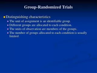
Today we will examine • Sample size determinants • Precision requirements • Sample allocation • Covariate adjustments • Matching and blocking • Subgroup analyses • Generalizing findings for sites and blocks • Using two-level data for three-level situations
Part I: The Basics
Statistical properties of group-randomized impact estimators Unbiased estimates Yij = a+B0Tj+ej+eij E(b0) = B0 Less precise estimates VAR(eij) = s2 VAR(ej) = t2 r = t2/(t2+s2)
Design Effect(for a given total number of individuals) ______________________________________ IntraclassIndividuals per Group (n) Correlation (r) 10 50 500 • 0.01 1.04 1.22 2.48 • 0.05 1.20 1.86 5.09 • 0.10 1.38 2.43 7.13 • _____________________________________
Sample design parameters • Number of randomized groups (J) • Number of individuals per randomized group (n) • Proportion of groups randomized to program status (P)
Reporting precision • A minimum detectable effect (MDE) is the smallest true effect that has a “good chance” of being found to be statistically significant. • We typically define an MDE as the smallest true effect that has 80 percent power for a two-tailed test of statistical significance at the 0.05 level. • An MDE is reported in natural units whereas a minimum detectable effect size (MDES) is reported in units of standard deviations
Minimum Detectable Effect SizesFor a Group-Randomized Design with r = 0.05 and no Covariates ___________________________________ Randomized Individuals per Group (n) Groups (J) 10 50 500 10 0.77 0.53 0.46 20 0.50 0.35 0.30 40 0.35 0.24 0.21 120 0.20 0.14 0.12 ___________________________________
Implications for sample design • It is extremely important to randomize an adequate number of groups. • It is often far less important how many individuals per group you have.
Part II Determining required precision
When assessing how much precision is needed: Always ask “relative to what?” • Program benefits • Program costs • Existing outcome differences • Past program performance
Effect Size Gospel According to Cohen and Lipsey Cohen Lipsey (speculative) (empirical) _______________________________________________ Small = 0.2s Small = 0.15s Medium = 0.5s Medium = 0.45s Large = 0.8s Large = 0.90s
Five-year impacts of the Tennessee class-size experiment Treatment: 13-17 versus 22-26 students per class Effect sizes: 0.11s to 0.22s for reading and math Findings are summarized from Nye, Barbara, Larry V. Hedges and Spyros Konstantopoulos (1999) “The Long-Term Effects of Small Classes: A Five-Year Follow-up of the Tennessee Class Size Experiment,” Educational Evaluation and Policy Analysis, Vol. 21, No. 2: 127-142.
Annual reading and math growth Reading Math Grade Growth Growth Transition Effect Size Effect Size ---------------------------------------------------------------- K - 1 1.52 1.14 1 - 2 0.97 1.03 2 - 3 0.60 0.89 3 - 4 0.36 0.52 4 - 5 0.40 0.56 5 - 6 0.32 0.41 6 - 7 0.23 0.30 7 - 8 0.26 0.32 8 - 9 0.24 0.22 9 - 10 0.19 0.25 10 - 11 0.19 0.14 11 - 12 0.06 0.01 ------------------------------------------------------------------------------------------------- Based on work in progress using documentation on the national norming samples for the CAT5, SAT9, Terra Nova CTBS, Gates MacGinitie (for reading only), MAT8, Terra Nova CAT, and SAT10. 95% confidence intervals range in reading from +/- .03 to .15 and in math from +/- .03 to .22
Performance gap between “average” (50th percentile) and “weak” (10th percentile) schools Source: District I outcomes are based on ITBS scaled scores, District II on SAT 9 scaled scores, District III on MAT NCE scores, and District IV on SAT 8 NCE scores.
Demographic performance gap in reading and math: Main NAEP scores Source: U.S. Department of Education, Institute of Education Sciences, National Center for Education Statistics, National Assessment of Educational Progress (NAEP), 2002 Reading Assessment and 2000 Mathematics Assessment.
Part III The ABCs of Sample Allocation
Sample allocation alternatives Balanced allocation • maximizes precision for a given sample size; • maximizes robustness to distributional assumptions. Unbalanced allocation • precision erodes slowly with imbalance for a given sample size • imbalance can facilitate a larger sample • Imbalance can facilitate randomization
Variance relationships for the program and control groups • Equal variances: when the program does not affect the outcome variance. • Unequal variances: when the program does affect the outcome variance.
Minimum Detectable Effect Size For Sample Allocations Given Equal Variances AllocationExample* Ratio to Balanced Allocation 0.5/0.5 0.54s 1.00 0.6/0.4 0.55s 1.02 0.7/0.3 0.59s 1.09 0.8/0.2 0.68s 1.25 0.9/0.1 0.91s 1.67 ________________________________________ * Example is for n = 20, J = 10, r = 0.05, a one-tail hypothesis test and no covariates.
Implications of unbalanced allocations with unequal variances
Implications Continued The estimated standard error is unbiased • When the allocation is balanced • When the variances are equal The estimated standard error is biased upward • When the larger sample has the larger variance The estimated standard error is biased downward • When the larger sample has the smaller variance
Interim Conclusions • Don’t use the equal variance assumption for an unbalanced allocation with many degrees of freedom. • Use a balanced allocation when there are few degrees of freedom.
References Gail, Mitchell H., Steven D. Mark, Raymond J. Carroll, Sylvan B. Green and David Pee (1996) “On Design Considerations and Randomization-Based Inferences for Community Intervention Trials,” Statistics in Medicine 15: 1069 – 1092. Bryk, Anthony S. and Stephen W. Raudenbush (1988) “Heterogeneity of Variance in Experimental Studies: A Challenge to Conventional Interpretations,” Psychological Bulletin, 104(3): 396 – 404.
Part IV Using Covariates to Reduce Sample Size
Basic ideas • Goal: Reduce the number of clusters randomized • Approach: Reduce the standard error of the impact estimator by controlling for baseline covariates • Alternative Covariates • Individual-level • Cluster-level • Pretests • Other characteristics
Impact Estimation with a Covariate yij = the outcome for student i from school j Tj = 1 for treatment schools and 0 for control schools Xj = a covariate for school j xij = a covariate for student i from school j ej = a random error term for school j eij = a random error term for student i from school j
Minimum Detectable Effect Size with a Covariate MDES = minimum detectable effect size MJ-K = a degrees-of-freedom multiplier1 J = the total number of schools randomized n = the number of students in a grade per school P = the proportion of schools randomized to treatment • = the unconditional intraclass correlation (without a covariate) R12 = the proportion of variance across individuals within schools (at level 1) predicted by the covariate R22 = the proportion of variance across schools (at level 2) predicted by the covariate 1 For 20 or more degrees of freedom MJ-K equals 2.8 for a two-tail test and 2.5 for a one-tail test with statistical power of 0.80 and statistical significance of 0.05
Questions Addressed Empirically about the Predictive Power of Covariates • School-level vs. student-level pretests • Earlier vs. later follow-up years • Reading vs. math • Elementary vs. middle vs. high school • All schools vs. low-income schools vs. low-performing schools
Empirical Analysis • Estimate r, R22 and R12 from data on thousands of students from hundreds of schools, during multiple years at five urban school districts • Summarize these estimates for reading and math in grades 3, 5, 8 and 10 • Compute implications for minimum detectable effect sizes
Estimated Parameters for Reading with a School-level Pretest Lagged One Year ___________________________________________________________________ School District ___________________________________________________________ A B C D E ___________________________________________________________________ Grade 3 r 0.20 0.15 0.19 0.22 0.16 R22 0.31 0.77 0.74 0.51 0.75 Grade 5 r 0.25 0.15 0.20 NA 0.12 R22 0.33 0.50 0.81 NA 0.70 Grade 8 r 0.18 NA 0.23 NA NA R22 0.77 NA 0.91 NA NA Grade 10 r 0.15 NA 0.29 NA NA R22 0.93 NA 0.95 NA NA ____________________________________________________________________
Minimum Detectable Effect Sizes for Reading with a School-Level Pretest (Y-1) or a Student-Level Pretest (y-1) Lagged One Year ________________________________________________________ Grade 3 Grade 5 Grade 8 Grade 10 ________________________________________________________ 20 schools randomized No covariate 0.57 0.56 0.61 0.62 Y-1 0.37 0.38 0.24 0.16 y-1 0.38 0.40 0.28 0.15 40 schools randomized No covariate 0.39 0.38 0.42 0.42 Y-1 0.26 0.26 0.17 0.11 y-1 0.26 0.27 0.19 0.10 60 schools randomized No covariate 0.32 0.31 0.34 0.34 Y-1 0.21 0.21 0.13 0.09 y-1 0.21 0.22 0.15 0.08 ________________________________________________________
Key Findings • Using a pretest improves precision dramatically. • This improvement increases appreciably from elementary school to middle school to high school because R22 increases. • School-level pretests produce as much precision as do student-level pretests. • The effect of a pretest declines somewhat as the time between it and the post-test increases. • Adding a second pretest increases precision slightly. • Using a pretest for a different subject increases precision substantially. • Narrowing the sample to schools that are similar to each other does not improve precision beyond that achieved by a pretest.
Source Bloom, Howard S., Lashawn Richburg-Hayes and Alison Rebeck Black (2007) “Using Covariates to Improve Precision for Studies that Randomize Schools to Evaluate Educational Interventions”Educational Evaluation and Policy Analysis, 29(1): 30 – 59.
Part VThe Putative Power of Pairing A Tail of Two Tradeoffs (“It was the best of techniques. It was the worst of techniques.” Who the dickens said that?)
Pairing Why match pairs? • for face validity • for precision How to match pairs? • rank order clusters by covariate • pair clusters in rank-ordered list • randomize clusters in each pair
When to pair? • When the gain in predictive power outweighs the loss of degrees of freedom • Degrees of freedom • J - 2 without pairing • J/2 - 1 with pairing
Deriving the Minimum Required Predictive Power of Pairing Without pairing With pairing Breakeven R2
The Minimum Required Predictive Power of Pairing Randomized Required Predictive Clusters (J) Power (R min2)* 6 0.52 8 0.35 10 0.26 20 0.11 30 0.07 *For a two-tail test.
A few key points about blocking • Blocking for face validity vs. blocking for precision • Treating blocks as fixed effects vs.random effects • Defining blocks using baseline information
Part VI Subgroup Analyses: Learning from Diversity
Purposes • To assess generalizability through description (by exploring how impacts vary) • To enhance generalizability through explanation (by exploring what predicts impact variation)
Considerations • Research protocol: Maximize ex ante specification through theory and thought to minimize ex post data mining. • Assessment criteria • Internal validity • Precision • Defining Features • Program characteristics • Randomized group characteristics • Individual characteristics
Defining Subgroups by The Characteristics of Programs • Based only on program features that were randomized • Thus one cannot use implementation quality
Defining Subgroups by Characteristics Of Randomized Groups • Types of impacts • Net impacts • Differential impacts • Internal validity • only use pre-existing characteristics • Precision • Net impact estimates are limited by reduced number of randomized groups • Differential impact estimates are triply limited (and often need four times as many randomized groups)
Defining Subgroups by Characteristics of Individuals • Types of impacts • Net impacts • Differential impacts • Internal validity • Only use pre-existing characteristics • Only use subgroups with sample members from all randomized groups • Precision • For net impacts: can be almost as good as for full sample • For differential impacts: can be even better than for full sample