Download
1 / 41
410 likes | 572 Views
Constraints – Finite Domains. Global Constraints for Scheduling Cumulative Flexible Tasks and Disjunction Placement Problems Spacial non-overlapping Placement vs. Scheduling Redundant Global Constraints. Global Constraints: cumulative.

E N D
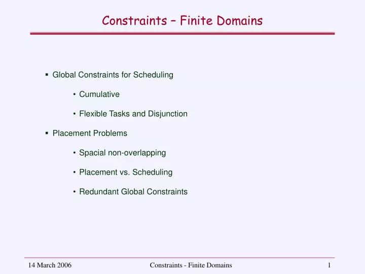
Constraints – Finite Domains • Global Constraints for Scheduling • Cumulative • Flexible Tasks and Disjunction • Placement Problems • Spacial non-overlapping • Placement vs. Scheduling • Redundant Global Constraints Constraints - Finite Domains
Global Constraints: cumulative • Global constraint serialized(T,D) that constrains the tasks with starting times in T and durations in D to be serialised, is just a special case of a more general global constraint cumulative(T,D,R,L) • For a set of tasks Ti, with duration Di and that use an amount Ri of some resource, this constraint guarantees that at no time there are more than L units of the resource being used by the tasks.. • The serialisation is imposed if each task uses 1 unit of a resource for which there is only that unit available, i.e. serialized(T,D) cumulative(T,D,R,1) where R = [1,1,...1]. Constraints - Finite Domains
Global Constraints: cumulative • The global constraint cumulative/4 allows not only to reason efficiently and globally about the tasks, but also to specify in a compact way this type of constraints, whose decomposition in simpler constraints would be very cumbersome. • Its semantics is as follows Let a = mini(Ti) ; b = maxi(Ti+Di); Si,k = Riif Ti =< tk =< Ti+Di or 0 otherwise. Then cumulative(T,D,R,L) Si,k L k[a,b] i Constraints - Finite Domains
Global Constraints: cumulative • This global constraint, cumulative/4, was initially introduced in the CHIP system CHIP [AgBe94] aiming at the efficient execution of a number of problems namely, • Schedulling of disjoint tasks • Schedulling of tasks with resource limitations • Placement problems • Its implementation is not presented in the article. A generalisation of this constraint, recently implemented in SICStus, allows positive and negative resource consumption to allow the modelling of producer consumer processes. Its implementation is explained in [BeCa02]. Constraints - Finite Domains
Global Constraints: cumulative • With constraint cumulative/4, the problem may be specified directly as in program schedule (predicate latest constrains all the tasks to end before the due time, Tmax). plan1(Tmax,Rmax, T):- T = [T1,T2,T3,T4,T5,T6,T7], D = [ 2, 4, 3, 2, 1, 2, 2], R = [ 4, 1, 3, 1, 2, 3, 2], domain(T, 1, 15), cumulative(T,D,R,Rmax), latest(T,D,Tmax), labeling([ff],T). • Note: The “area” of all the tasks is 35, so the problem is only possible if Tmax * Rmax >= 35 Constraints - Finite Domains
Global Constraints: cumulative Example: Take 7 tasks (A a G) with the duration and resource consumption (e.g. number of workers needed to carry them out) specified in the following lists D = [ 2 , 4 , 3 , 2 , 1 , 2 , 2 ] ; R = [4 , 1 , 3 , 1 , 2 , 3 , 2 ] Find whether the tasks may all be finished in a given due time Tmax, assuming there are Rmax resources (e.g. Workers) available at all times. Graphically, the tasks can be viewed as Constraints - Finite Domains
R t Global Constraints: cumulative Results With Tmax = 9 and Rmax = 4 a number of answers are obtained, namely Constraints - Finite Domains
Global Constraints: cumulative Results With Tmax = 7 and Rmax = 5 (in this case, no resources may be spared), a number of answers are still obtained, such as Constraints - Finite Domains
Global Constraints: cumulative Results With Tmax = 6 and Rmax = 6 (in this case, one of the 6 workers may rest for an hour), still a number of answers are obtained, namely Question:What about Tmax = 5 e Rmax = 7 ? Constraints - Finite Domains
Flexible Tasks in Scheduling • In some applications, tasks are flexible, in the sense that time may be traded for resources. • For example, a flexible task might require either 2 workers working for 3 hours, or 3 workers working for 2 hours. It may even be executed by a single worker during 6 hours, or by 6 workers in 1 hour. • Flexible tasks may be more easily accomodated within the resources (and time) available. • Scheduling of this type of tasks may be specified as before. However, whereas in the previous case, the durations and resources were constants Kdi e Kri , the durations Di and resources Ri of flexible tasks must be constrained by Di * Ri #= Kdi * Kri Constraints - Finite Domains
Flexible Tasks in Scheduling • The program below is similar to the previous, but imposes flexibility on tasks with predicate constrain_tasks/2. Of course, since both the durations and resources are now variables, labelling must be made in (one of) such variables. plan2(Tmax,Rmax, T, D, R):- T = [T1,T2,T3,T4,T5,T6,T7], domain([T1,T2,T3,T4,T5,T6,T7], 1, 15), D = [D1,D2,D3,D4,D5,D6,D7], Dc = [ 2, 4, 3, 2, 1, 2, 2], R = [R1,R2,R3,R4,R5,R6,R7], Rc = [ 4, 1, 3, 1, 2, 3, 2], constrain_tasks(D,R,Dc,Rc), cumulative(T,D,R,Rmax), latest(T,D,Tmax), append(T,D,V), labeling([ff],V). Constraints - Finite Domains
Flexible Tasks in Scheduling • Predicate constrain_tasks/2 is implemented as shown below. Variables D and R are assigned initial domains 1..9 , and for each task, the constraint specifying flexibility is imposed. constrain_tasks(D,R,Dc,Rc):- domain(D, 1, 9), domain(R, 1, 9), set_cons(D,R,Dc,Rc). set_cons([],[],[],[]). set_cons([D1|Dt1],[R1|Rt1],[D2|Dt2],[R2|Rt2]):- D1 * R1 #= D2 * R2, set_cons(Dt1,Rt1,Dt2,Rt2). Constraints - Finite Domains
Global Constraints: cumulative Results With Tmax = 6 and Rmax = 6 (in this case, one of the 6 workers may rest for an hour), still a number of answers are obtained, namely Constraints - Finite Domains
Global Constraints: cumulative Results With Tmax = 6 and Rmax = 6 (in this case, one of the 6 workers may rest for an hour), still a number of answers are obtained, namely Constraints - Finite Domains
Scheduling and Cumulative Constraint: Job-Shop • The job shop problem consists of executing the different tasks of several jobs without exceeding the available resources. • Within each job, there are several tasks, each with a duration. Within each job, the tasks have to be performed in sequence, possibly respecting mandatory delays between the end of a task and the start of the following task. • Tasks of different jobs are independent, except for the sharing of common resources (e.g. machines). • Each task must be executed in a machine of a certain type. The number of machines of each type is limited. Constraints - Finite Domains
Scheduling and Cumulative Constraint: Job-Shop • Denoting by JXYZ the Y-th task of job X, to be executed in machine Z, with duration D, an instance of the 10*10 job-shop is shown in the following table Constraints - Finite Domains
Scheduling and Cumulative Constraint: Job-Shop History • This instance was proposed in the book Industrial Scheduling [MuTh63]. • For 20 years no solution was found that optimised the “makespan”, i.e. the fastest termination of all tasks. • Around 1980, the best solution was 935 (time units). In 1985, the optimum was lower bounded to 930. • In 1987 the problem was solved with a highly specialised algorithm, that found a solution with makespan 930. • With the cumulative/4 constraint, in the early 1990’s, the problem was solved in 1506 seconds (in a SUN/SPARC workstation). Constraints - Finite Domains
Scheduling and Cumulative Constraint: Job-Shop • A simpler instance of the problem is given in the table below (with the corresponding graphic representation). • Notice that in this instance it is assumed that each task requires one unit of the resource shown, and that there are 2 units of resource 1 and other 2 units of resource 2. Constraints - Finite Domains
Scheduling and Cumulative Constraint: Job-Shop • This instance of the problem may be easily solved by the following SICStus program (see file jobshop): jobs([J1,J2,J3,J4]):- % definition of the jobs J1 = [S111,S122,S131]-[2,4,7]-[1,2,1], J2 = [S211,S222,S231]-[3,4,5]-[1,2,1], J3 = [S311,S322,S332]-[5,3,3]-[1,2,2], J4 = [S411,S422,S432]-[3,3,4]-[1,2,2], % domain declarations domain([S111,S122,S131],0,15), domain([S211,S222,S231],0,15), domain([S311,S322,S332],0,15), domain([S411,S422,S432],0,15), % precedence constraints % resource limitation contraints % constraints on the end of the jobs % labelling of the tasks starting times Constraints - Finite Domains
Scheduling and Cumulative Constraint: Job-Shop The constraints are as follows: % precedence constraints S122#>=S111+2, S131#>=S122+4, S222#>=S211+3, S231#>=S222+4, S322#>=S311+5, S332#>=S322+3, S422#>=S411+3, S432#>=S422+3, % resource limitation contraints cumulative([S111,S131,S211,S231,S311,S411], [2,7,3,5,5,3], [1,1,1,1,1,1],2), cumulative([S122,S222,S322,S332,S422,S432], [4,4,3,3,3,4], [1,1,1,1,1,1],2), % constraints on the end of the jobs E #>= S131+7, E #>= S231+5, E #>= S332+3, E #>= S432+4, E #=< 13, % labelling of the tasks starting times labeling([ff],[S111, S122, S131, S211, S222, S231, S311, S322, S332, S411, S422, S432]). Constraints - Finite Domains
Scheduling and Cumulative Constraint: Job-Shop The possible results, with termination no later than 13, are the following : | ?- jobs(J). J=[[0,2, 6]-[2,4,7]-[1,2,1],[0,3,7]-[3,4,5]-[1,2,1], [2,7,10]-[5,3,3]-[1,2,2],[3,6,9]-[3,3,4]-[1,2,2]]?; J=[[0,2, 6]-[2,4,7]-[1,2,1],[0,3,8]-[3,4,5]-[1,2,1], [2,7,10]-[5,3,3]-[1,2,2],[3,6,9]-[3,3,4]-[1,2,2]]?; no Constraints - Finite Domains
Placement Problems • Several applications of great (economic) importance require the satisfaction of placement constraints, i.e. the determination of where to place a number of components in a given space, without overlaps. Some of these applications include: • Wood boards cuttings, where a number of smaller pieces should be taken from large boards: • Similar problem in the textil context; • Placement of items into a large container. • In the first 2 problems the space to consider is 2D, whereas the third problem is a typical 3D application. We will focus on 2D problems. Constraints - Finite Domains
Placement Problems • An immediate parallelism can be drawn between these 2D problems and those of scheduling, if the following correspondences are made: • Time the X dimension; • Resources the Y dimension; • A task duration the item X size (width); • A task resource the item Y size (height). • Hence, the problems used before should apparently be used for this new kind of problems, with the above adaptations. Constraints - Finite Domains
Placement Problems Example: Find the appropriate cuts to be made on a wood board so as to obtain 11 rectangular pieces (A a K). The various pieces to obtain have the following dimensions (width-W and height-H) W = [ 1, 2, 1, 3, 1, 2, 4, 5, 2, 3, 3] H = [ 2, 1, 3, 1, 4, 2, 1, 1, 3, 2, 3] Graphically Constraints - Finite Domains
Placement Problems Example: Find the appropriate cuts to be made on a wood board so as to obtain 11 rectangular pieces (A a K). The various pieces to obtain have the following dimensions (width-W and height-H) W = [ 1, 2, 1, 3, 1, 2, 4, 5, 2, 3, 3] H = [ 2, 1, 3, 1, 4, 2, 1, 1, 3, 2, 3] Graphically Constraints - Finite Domains
Placement Problems This problem can be thus specified as below place(Width, Height):- % rectangles definition X = [Ax,Bx,Cx,Dx,Ex,Fx,Gx,Hx,Ix,Jx,Kx], W = [ 2, 1, 1, 3, 1, 2, 4, 5, 2, 3, 3], H = [ 1, 2, 3, 1, 4, 2, 1, 1, 3, 2, 3], domain(X, 1, Width), % constraints in X-origins maximum(X,W,Width), cumulative(X,W,H,Height), % enumeration of rectangles X-origin labeling([ffc], X). Constraints - Finite Domains
Placement Problems • Unfortunately, the results obtained have not a direct reading. For example, one of the solutions obtained with an 8*6 rectangle is X = [ 6, 7, 5, 1, 4, 5, 1, 1, 7, 6, 1] That can be read as (???) or as Constraints - Finite Domains
Placement Problems • To avoid this ambiguity, one should explicitely compute, not only the X-origin of the rectangles, but also its Y-origin. • Such computation can easily be made, taking into account that all that is needed is considering a rotation of 90º in the viewing perspective, changing the X with the Y axes. • Hence, all that is required is a “duplication” of the previous program, considering not only X variables, but also Y variables for explicit control over the Y-origins of the rectangles. Constraints - Finite Domains
Placement Problems • Firstly, new Y variables are created place(Width,Height):- % rectangles definition X = [Ax,Bx,Cx,Dx,Ex,Fx,Gx,Hx,Ix,Jx,Kx], Y = [Ay,By,Cy,Dy,Ey,Fy,Gy,Hy,Iy,Jy,Ky], W = [ 2, 1, 1, 3, 1, 2, 4, 5, 2, 3, 3], H = [ 1, 2, 3, 1, 4, 2, 1, 1, 3, 2, 3], domain(X, 1, Width), domain(Y, 1, Height), % constraints in X- and Y-origins ... % enumeration of rectangles X- and Y origins ... Constraints - Finite Domains
Placement Problems • Secondly, similar constraints (but with a 90º rotation) are imposed on them place(Width,Height):- % rectangles definition ... % constraints in X- and Y-origins maximum(X,W,Width), cumulative(X,W,H,Height), maximum(Y,H,Height), cumulative(Y,H,W,Width), % enumeration of rectangles X- and Y- origins labeling([ffc], X), labeling([ffc], Y). Constraints - Finite Domains
????? Placement Problems • Yet, the results still aren’t what they should be. For example, the first solution obtained is X-Y = [7-4,6-2,5-1,1-5,4-1,5-4,1-1,1-6,7-1,6-5,1-2] corresponding to • Analysing the problem, it becomes clear that its cause is the fact that no non-overlaping constraint was imposed on the rectangles! Constraints - Finite Domains
Placement Problems • The non overlapping of the rectangles defined by their Xi and Yi origins and their widths Wi (X-sizes) and heights Hi (Y sizes) is guaranteed, as long as one of the constraints below is satisfied (for rectangles 1 and 2) X1+W1 =< X2Rectangle 1 is to the left of 2 X2+W2 =< X1Rectangle 1 is to the rigth of 2 Y1+H1 =< Y2Rectangle 1 is below 2 Y2+H2 =< Y1Rectangle 1 is above 2 • As explained before, rather than commiting to one of these conditions, and change the commitment by backtracking, a better option is to adopt a least commitment approach, for example with some kind of “cardinality” meta-constraint. Constraints - Finite Domains
Placement Problems Important points to stress • The enumeration should be made jointly on both the Xi and the Yj, hence their merging into a single list Z. • Several heuristics could possibly be used for variable enumeration. The heuristic chosen, ffc, is the classical choice. • Alternatively, one could possibly start placing the “largest” rectangles in the corners, so as to make room for the others. • The Cumulative constraints are not strictly necessary, given the overlapping and the maximum constraints applied in both dimensions. • Yet, they are extremely useful. Without them, the program would “hardly” work! Constraints - Finite Domains
Placement Problems • The program for the placement problem, place_1, showing the simetry on the X and Y axes, is presented below. place(Width,Height):- % rectangles definition X = [Ax ... Kx], Y = [Ay ... Ky], W = [ 1 ... 3], H = [ 2 ... 3], domain(X, 1, Width), domain(Y, 1, Heigth), % constraints on X and Y origins maximum(X,W,Width), maximum(Y,H,Heigth), % redundant cumulative constraints cumulative(Y,H,W,Width), cumulative(X,W,H,Height), % non overlapping constraints none_overlap(X,Y,D,R), % joint enumeration of X and Y origins app(X,Y,Z), labeling([ffc], Z). Constraints - Finite Domains
Placement Problems • The results obtained show well the importance of using the redundant cumulative/4 constraints. Testing the program presented with and without these constraints, the following results are obtained in 16 ms in 5.407 s with cumulative without cumulative Constraints - Finite Domains
Placement Problems with Rotation • An obvious limitation of the program shown is its impossibility to “rotate” the components by 90º for better accomodation in the available space. • Sometimes, a placement is only possible if these rotations are performed in some of the components. • The changes to make in the program are small. Given constant dimensions Ac - Bc, it must be guaranteed that they are either interpreted as Width-Height or as its Height-Width . • Given the fixed dimensions, such flexibility is obtained by simple constructive disjunction, and user controled by means of parameter Mode (fix/rot) disallowing or allowing rotations, respectively. Constraints - Finite Domains
Placement Problems with Rotation Example: ... Wc = [ 6, 6, 5, 5, 4, 4, 3, 3, 2, 2], Hc = [ 2, 1, 2, 1, 2, 1, 2, 1, 2, 1], domains(Mode,W,H,Wc,Hc), ... ======================= domains(fix, [],[],[],[]). domains(fix, [W|Wt],[H|Ht],[Wc|Wtc],[Hc|Htc]):- W = Wc, H = Hc, domains(fix,Td,Tr,Tdc,Trc). domains(rot, [],[],[],[]). domains(rot,[Hd|Td],[Hr|Tr],[Hdc|Tdc],[Hrc|Trc]):- Hd in {Hdc}\/{Hrc}, Hr in {Hdc}\/{Hrc}, Hr * Hd #= Hdc * Hrc, domains(rot, Td,Tr,Tdc,Trc). Constraints - Finite Domains
Placement Problems with Rotation • The labeling of these new variables W and H must now be considered in the enumeration. In fact, only one set of these variables requires enumeration, since the other is automatically computed. • A possible heuristic to be used is to label the most difficult rectangles first. Here we consider that the difficulty of placing the rectangles depends on their largest dimension. Hence we sort them in the merge predicate and label them in this order (no ffc). • Only after enumerating the rectangles we enumerate the rotations, for the case they had not been set yet. merge( X, Y, Z), labeling([], Z), labeling([ffc], W), Constraints - Finite Domains
Placement Problems with Rotation Example: 10 rectangles (A to J) must be cut from a wood board with rectangular shape, with total area of 60, rotations being allowed for better accomodation of the rectangles. The rectangles have the following dimensions (width-W and height-H) Wc = [ 6, 6, 5, 5, 4, 4, 3, 3, 2, 2], Hc = [ 2, 1, 2, 1, 2, 1, 2, 1, 2, 1], Graphically, Constraints - Finite Domains
Placement Problems with no Rotation Results obtained (see place_2): Fix mode : Constraints - Finite Domains
Placement Problems with Rotation Results obtained (see place_2): Rot mode : Constraints - Finite Domains