Download
1 / 53
550 likes | 783 Views
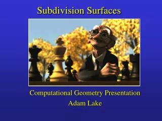
Subdivision Surfaces. Computational Geometry Presentation Adam Lake. Motivation. Scalability across machines Speed of evaluation LOD in a scene Topological restrictions of NURBS surfaces Planes, Cylinders, and Torii. Motivation. Trimming is expensive and prone to numerical error

E N D
Subdivision Surfaces Computational Geometry Presentation Adam Lake
Motivation • Scalability across machines • Speed of evaluation • LOD in a scene • Topological restrictions of NURBS surfaces • Planes, Cylinders, and Torii
Motivation • Trimming is expensive and prone to numerical error • It is difficult to maintain smoothness at seams of patchwork. • Example: hiding seams in Woody (Toy Story) [DeRose98] • Advantage of NURBS: Trimmed NURBS are readily available in commercial systems!!
Subdivisions of Talk • 2D and 3D Examples • Give data structure for geometry • Define B-spline curve • Derive splitting matrix for bicubics • Define arbitrary topology splitting rules • Define extraordinary vertices, Doo-Sabin surfaces
2D subdivision curve example • De Casteljau curve [Foley90] P2 P3 P4 P1
2D subdivision curve example • De Casteljau curve [Foley90] H=(P2+P3)/2 P2 P3 L3=(L2+H)/2 R2=(H+R3)/2 L2=(P1+P2)/2 L4=R1=(L3+R2)/2 R3=(P3+P4)/2 P4=R4 P1=L1
Major categories of subdivision surfaces • Catmull-Clark [Catmull78] • Doo-Sabin [Doo78] • Loop [Loop87] • Butterfly scheme [Dyn90]
Subdivision Surface Data Structure A mesh is a pair (K,V) where K is a simplical complex representing connectivity of the vertices, edges, and faces. Determines topological type of the mesh. V={v1,v2,v3…vn}, vi in R^3 is a set of vertex positions defining the shape of the mesh in R^3. Example: V={[0,0,0],[1,0,0],[0,0,1]} Simplical complex K: vertices: {1},{2},{3} edges: {1,2},{2,3},{1,3} faces: {1,2,3} 2 1 3
B-Spline Patch Splitting The Bicubic B-Spline Patch can be expressed as: Where:
B-Spline Patch Splitting • Now, consider a subdivision scheme for 0<=u,v<=1/2 and introduce a matrix • In order to obtain the same patch we must have:
B-Spline Patch Splitting • Assuming M is invertible: This is known as the splitting matrix. Note: Mistake in original paper!!!
p41 p42 p43 p44 p34 p24 p12 p13 p14 p11 q12 q11 q22 q21 B-Spline Patch Splitting p31 p21
p41 p42 p43 p44 p34 p24 p12 p13 p14 p11 q12 q11 q22 q21 B-Spline Patch Splitting p11
Arbitrary Topology • 3 types of points • Face • Edge • Vertex • Edges formed by 2 rules • Subdivision surface is the LIMIT surface
Arbitrary Topology • New face points • Average of all old points defining the face. • Example
Arbitrary Topology • New edge points • Average midpoints of old edge with average of the two new face points of faces sharing edge • Example
Arbitrary Topology • New vertex points • Q=average of the new face points of all faces adjacent to the old vertex point • R=average of the midpoints of all old edges incident on the old vertex points • S=old vertex point
Arbitrary Topology • New edges formed by: • Connecting each new face point to new edge points of edges defining the old face • Connecting each new vertex point to the new points of all old edges incident to old vertex point • Example
Extraordinary points • Previous method generates continuous surfaces except at extraordinary points • Extraordinary points have valence other than 4 N=5 N=3 Extraordinary points
Doo-Sabin Surfaces • Doo-Sabin showed via Eigenanalysis that at extraordinary points the surface is discontinuous and proposed modified rules to maintain continuity in the surface [Doo78]. • The improved formulation is known as Doo-Sabin surfaces.
Bi-quadratic surfaces • Applying the method for bi-cubic can also be used to derive bi-quadratic surfaces.
Recap • So far: • 2D and 3D examples • Data structure for geometry • Defined B-spline curve • Derived the splitting matrix for bicubics • Defined arbitrary topology splitting rules • Defined extraordinary vertices, Doo Sabin surfaces
Next • Subdivision surfaces in Character Animation [DeRose98] • Non-uniform Subdivision Surfaces [Sederberg98] • Exact Evaluation of Catmull Clark surfaces at arbitrary parameter values [Stam98] • MAPS: Multiresolution Adaptive Parameterization of Surfaces [Lee98]
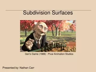
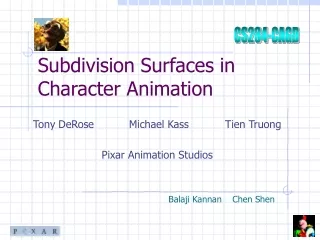
Subdivision Surfaces in character animation [DeRose98] • Used for first time in Geri’s game to overcome topological restriction of NURBS • Modeled Geri’s head, hands, jacket, pants, shirt, tie, and shoes • Developed cloth simulation methods • Method to construct scalar fields enabling use of programmable shaders
Why Catmull-Clark? • Quads are better than tris at capturing the symmetries of natural and man-made objects. Tube like surfaces (arms, legs, fingers) are easier to model. • Generalize uniform tensor product cubic B-splines, makes it easier to use in-house and commercial systems (Renderman and Alias-Wavefront).
Hybrid subdivision • Hoppe wrote about smooth surfaces with infinitely sharp creases. • DeRose generalizes this to semi-sharp creases • Select certain vertices to use rules to subdivide to a specific level, then switch to another subdivision scheme applied to the limit. • Sharp at coarse scales, smooth at finer scales • Calls this hybrid subdivision
Subdivision Surfaces in character animation • Implemented in Renderman • Shows subdivision surfaces can be used in high end rendering
Non-uniform subdivision surfaces [Sederberg98] • For a non-uniform surface, each vertex is assigned a knot spacing that may be different from each edge radiating from it. • If all knot intervals are equal, back to regular Catmull-Clark or Doo-Sabin. [Cannot be represented as NURB nor uniform Catmull Clark]
Exact Evaluation of Catmull-Clark Surfaces at arbitrary parameter values [Stam98]
Exact Evaluation of Catmull-Clark Surfaces at arbitrary parameter values [Stam98] • Disproves belief that Catmull Clark surfaces cannot be evaluated w/o explicit subdividing. • Uses a set of eigenbasis functions and derive analytical expressions for these functions. • Cost comparable to that of a bi-cubic B-spline. • Allows algorithms developed for parametric surfaces to be applied to Catmull-Clark surfaces.
First high resolution plots around regions of high curvature Extraordinary point in center. Patches using technique are in blue. Derivative information is computed and displayed in model on right.
MAPS: Multiresolution Adaptive Parameterization of Surfaces [Lee98]
MAPS: Multiresolution Adaptive Parameterization of Surfaces [Lee98] Note: Great computational geometry paper!!
Step 1:A scanned input mesh • Acquired via laser range scanning or MRI volumetric imaging followed by isosurface extraction • Arbitrary topology • Irregular structure • Tremendous size
Step 2: Via mesh simplification, obtain the parameter or base domain • During simplification, building a topological representation for O(nlgn) multiresolution representation.
Step 2: Via mesh simplification, obtain the parameter or base domain
Step 3: Assign triangles in original mesh to their base domain triangle (during 1->2) + =
Step 4: Adaptive Remeshing with subdivision connectivity (epsilon = 1%) Uniform mesh obtained via Loop scheme Interested insmooth parameterizations, not simplification!!
Step 4 (detail)Motivation • Assume a smooth parameterization within each subdomain (see paper for details) • One way to obtain global smoothness would be to minimize a global smoothness functional. • Requires PDE solver. • Found that this is needlessly cumbersome. • Instead, use simpler and cheaper smoothing technique based on Loop subdivision.
Step 4 (detail)Modified Loop Scheme • If all points of stencil needed for computing new point or smoothing old point are inside same triangle of base domain, add Loop weights and new points will be in the same face • If stencil stretches across 2 faces, flatten using hinge map at common edge. • If stencil stretches across multiple faces, use a conformal flattening strategy (see paper).
Step 4 (details) Smoothed mesh using modified Loop simplification scheme
Step 5: Multiresolution editing Smooth parameterization allows efficient mesh modification. Texture coordinates and polygons nicely behaved.
Summary • Who developed them? • Catmull-Clark • Doo-Sabin • Loop • Dyn (butterfly) • Recent work • DeRose, Sederberg, Lee, Stam
Summary • What are they? • Mesh based representation of geometry • Defined recursively • Many levels of fidelity
Summary • Where can they be used? • Animation • CAD modeling • Game engines • more?