Download
1 / 20
300 likes | 716 Views
A. +. +. +. +. +. I. CHAPTER 27 : CURRENT AND RESISTANCE 27.1) ELECTRIC CURRENT A system of electric charges in motion. Whenever there is a net flow of charge through some region, a current is said to exist. To define current :

E N D
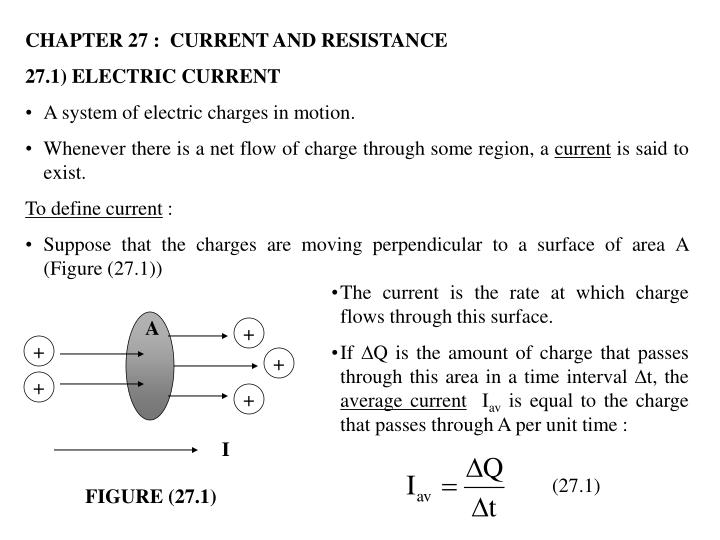
A + + + + + I • CHAPTER 27 : CURRENT AND RESISTANCE • 27.1) ELECTRIC CURRENT • A system of electric charges in motion. • Whenever there is a net flow of charge through some region, a current is said to exist. • To define current : • Suppose that the charges are moving perpendicular to a surface of area A (Figure (27.1)) • The current is the rate at which charge flows through this surface. • If Q is the amount of charge that passes through this area in a time interval t, the average current Iav is equal to the charge that passes through A per unit time : (27.1) FIGURE (27.1)
(27.2) (27.3) • If the rate at which charge flows varies in time, then the current varies in time; we define the instantaneous current I as the differential limit of average current : • The SI unit of current is the ampere (A) : • That is, 1A of current is equivalent to 1C of charge passing through the surface area in 1s. • The charges passing through the surface in Figure (27.1) can be positive or negative, or both. • It is conventional to assign to the current the same direction as the flow of positive charge. • The direction of the current is opposite the direction of flow of electrons. • A bean of positively charged protons in an accelerator – the current is in the direction of motion of the protons. • Involving gases and electrolytes – the current is the result of the flow of both positive and negative charges.
If the ends of a conducting wire are connected to form a loop • All points on the loop are at the sme electric potential. • Hence, the electric field is zero within and at the surface of the conductor. • Because the electric field is zero, no net transport of charge through the wire. • Therefore, no current. • The current in the conductor is zero even if the conductor has an excess of charge on it. • If the ends of the conducting wire are connected to a battery • All point on the loop are not at the same potential. • The battery sets up a potential difference between the ends of the loop. • Creating an electric field within the wire. • The electric field exerts forces on the conduction electrons in the wire. • Causing the electons to move around the loop. • Thus, creating current. • A moving charge (+ve or –ve) is a mobile charge carrier. • For example, the mobile charge carriers in a metal are electrons.
Microscopic Model of Current • We can relate current to the motion of the charge carriers by describing a microscopic model of conduction in a metal. • The current in a conductor of cross-sectional area A – Figure (27.2) • The volume of a section of the conductor of length x is A x (the gray region). • If n represents the number of mobile charge carriers per unit volume (the charge carrier density), the number of carriers in the gray section is n A x . • The charge Q in this section is : • Q =number of carriers in section charge per carrier = (n A x )q • where q = the charge on each carrier. • If the carriers move with a speed d, the distance they move in a time t is : x = d t. • Therefore, we can write Q in the form : Q = (nAd t)q FIGURE (27.2)
(27.4) • Example (27.1) : Drift Speed in a Copper Wire • The 12-gauge copper wire in a typical residential building has a cross-sectional area of 3.31 10-6 m2. If it carries a current of 10.0A, what is the drift speed of the electrons? Assume that each copper atom contributes one free electron to the current. The density of copper is 8.95 g/cm3. • Solution • From the periodic table of the elements in Appendix C, we find that the molar mass of copper 63.5 g/mol. • Recall that 1 mol of any substance contains Avogadro’s number of atoms (6.02x10²³). • If we devide both sides of this equation by t, we see that the average current in the conductor is : • The speed of the charge carriers d = an average speed called the drift speed.
Solution (continue) • Knowing the density of copper, we can calculate the volume occupied by 63.5 g (=1 mol) of copper. • Because each copper atom contributes one free electron to the current, we have : • From equation (27.4), we find that the drift speed is : where q is the absolute value of the charge on each electron. • Thus,
(27.5) • 27.2) RESISTANCE AND OHM’S LAW • In chapter 24, we found that no electric field can exist inside a conductor. • This statement is true only if the conductor is in static equilibrium. • What happens when the charges in the conductor are allowed to move? • Charges moving in a conductor produce a current under the action of an electric field, which is maintained by the connection of a battery across the conductor. • An electric field can exist in the conductor because the charges in this situation are in motion – that is, this is a nonelectrostatic situation. • Consider a conductor of cross-sectioned area A carrying a current I. • The current density J in the conductor is defined as the current per unit area. • Because the current I = nqdA, the current density is : • where J has SI units of A/m2.
This expression is valid only if i) the current density is uniform and only if ii) the surface of cross-sectional area A is perpendicular to the direction of the current. • In general, the current density is a vector quantity : • From Equation (27.6) – current density, like current, is in the direction of charge motion for positive charge carriers and opposite the direction of motion for negative charge carriers. • A current density and an electric field are established in a conductor whenever a potential difference is maintained across the conductor. • If the potential difference is constant, then the current also is constant. • In some materials, the current density is proportional to the electric field : • where the constant of proportionality is called the conductivity of the conductor. • Materials that obey Equation (27.7) are said to follow Ohm’s Law. (27.6) (27.7)
Ohm’s Law states that : For many materials (including most metals), the ration of the current density to the electric field is a constant that is independent of the electric field producing the current. • Materials that obey Ohm’s Law and hence demonstrate this simple relationship between and are said to be ohmic. • Not all materials have this property. • Materials that do not obey Ohm’s Law are said to be nonohmic. • To obtain a form of Ohm’s Law useful in practical applications • Consider a segment of straight wire of uniform cross-sectional area A and length as shown in Figure (27.5). I A Vb Va E FIGURE (27.5)
A potential difference V = Vb – Va is maintained across the wire, creating in the wire an electric field and a current. • If the field is assumed to be uniform, the potential difference is related to the field through the relationship • Therefore, we can express the magnitude of the current density in the wire as : • Because J = I/A, we can write the potential difference as : • The quantity is called the resistance R of the conductor.
We can define the resistance as the ratio of the potential difference across a conductor to the current through the conductor : • From this result we see that resistance has SI units of volts per ampere. • One volt per ampere is defined to be 1 ohm () : • Shows that : If a potential difference of 1V across a conductor causes a current of 1A, the resistance of the conductor is 1 . • The inverse of conductivity is resistivity : • where has the units ohm-meters (.m). • From Equations (27.8) and (27.10), the resistance of a uniform block of material is : (27.8) (27.9) (27.10) (27.11)
103 2 5% 0 red orange black gold • Notes • Characteristic resistivity depends on i) properties of the materials and ii) temperature. • Resistance of a sample depends on i) geometry and ii) resistivity. • Refer Table (27.1) page 847 – for value of resistivity, and temperature coefficient, . • Resistors • Use to control the current level in the various parts of the circuit. • Resistors’ values in ohms – indicated by color-coding (Table (27.2)). Table (27.2) : Color Coding for Resistors Tolerance value = 5% = 1k
I I Slope = 1/R V V (a) (b) • Ohmic materials have a linear current-potential difference relationship (Figure (27.7a)). • Non-ohmic materials have a nonlinear current-potential difference relationship (Figure (27.7b)). FIGURE (27.7)
Example (27.2) : Resistance of a Conductor Calculate the resistance of an aluminum cylinder that is 10.0 cm long and has a cross-sectional area of 2.00x10⁻⁴m2. Repeat the calculation for a cylinder of the same dimensions and made of glass having a resistivity of 3.0x1010.m. Solution From Equation (27.11) and Table (27.1), we can calculate the resistance of the aluminum cylinder as follows : Similarly, for glass we find that :
Example (27.3) : The Resistance of Nichrome Wire • Calculate the resistance per unit length of a 22-gauge Nichrome wire, which has a radius of 0.321 mm. • Solution : The cross-sectional area of this wire is • A = r2 = (0.321 x 10⁻³m)2 = 3.24 x 10⁻⁷ m2 • The resistivity of Nichrome is 1.5 x 10⁻⁶ .m (see Table (27.1)). • Thus, we can use Equation (27.11) to find the resistance per unit length : • (b) If a potential difference of 10V is maintained across a 1.0-m length of the Nichrome wire, what is the current in the wire? • Solution : Because a 1.0-m length of this wire has a resistance of 4.6, Equation (27.8) gives :
Example (27.4) : The Radial Resistance of a Coaxial Cable • Coaxial cables are used extensively for cable television and other electronic applications. A coaxial cable consists of two cylindrical conductors. The gap between the conductors is completely filled with silicon, as shown in Figure (27.8a), and current leakage through the silicon is unwanted. (The cable is designed to conduct current along its length). The radius of the inner conductor is a = 0.500cm, the radius of the outer one is b = 1.75cm, and the length of the cable is L = 15.0cm. Calculate the resistance of the silicon between the two conductors. • Solution • Divide the object whose resistance we are calculating into concentric elements of infinitesimal thickness dr (Figure (27.8b)). • We start by using the differential form of Equation (27.11), replacing with r for the distance variable : where dR is the resistance of an element of silicon of thickness dr and surface area A. FIGURE (27.8)
Solution (continue) • In this example, we take as our representative concentric element a hollow silicon cylinder of radius r, thickness dr, and length L, as shown in Figure (27.8) • Any current that passes from the inner conductor to the outer one must pass radially through this concentric element, and the area through which this current passes is A = 2 r L. (This is the curved surface area – circumference multiplied by length – of our hollow silicon cylinder of thickness dr.) • Hence, we can write the resistance of our hollow cylinder of silicon as : • Because we wish to know the total resistance across the entire thickness of the silicon, we must integrate this expression from r = a to r = b : • Substituting in the values given, and using = 640 .m for silicon, we obtain :
(27.19) (Variation of with temperature) (27.20) • 27.4) RESISTANCE AND TEMPERATURE • Over a limited temperature range, the resistivity of a metal varies approximately linearly with temperature according to the expression : • where • = the resistivity at some temperature T (in degrees Celsius), • o = the resistivity at some reference temperature To(usually taken to be 20oC). • = the temperature coefficient of resistivity. • From Equation (27.19), the temperature coefficient of resistivity can be expressed as : • where = - o is the change in resistivity in the temperature interval T= T – To.
(27.21) • The temperature coefficients of resistivity for various materials – Table (27.1). • The unit for is degrees Celsius-1 [ ( oC )-1 ] • Resistance is propotional to resistivity (Equation (27.11)) – the variation of resistance : Example (27.6) : A Platinum Resistance Thermometer A resistance thermometer, which measures temperature by measuring the change in resistance of a conductor, is made from platinum and has a resistance of 50.0 at 20.0oC. When immersed in a vessel containing melting indium, its resistance increases to 76.8 . Calculate the melting point of the indium. Solution Solving Equation (27.21) for T and using the value for platinum given in Table (27.1), we obtain :
Solution (continue) • Because To = 20.0oC, we find that T, the temperature of the melting indium sample, is 157oC. • Metals (e.g. copper) - resistivity is nearly proportional to temperature (Figure (27.10)). • - characterized by collisions between electrons and metal atoms. • However - a nonlinear region always exists at very low temperatures. • - the resistivity usualy approaches some finite value as the temperature nears absolute zero caused by the collision of electrons with impurities and imperfections in the metal. FIGURE (27.10)