Download

1 / 48
480 likes | 643 Views
Climate Forcings , Feedbacks, and Future Responses. Review of last lecture. Temperature conditions and climate on Earth are constrained by the balance between absorbed solar radiation and outgoing terrestrial radiation.

E N D
Review of last lecture • Temperature conditions and climate on Earth are constrained by the balance between absorbed solar radiation and outgoing terrestrial radiation. • The greenhouse effect is a synonym for the trapping of infrared radiation by radiatively active atmospheric constituents, which (for a given temperature) reduce the rate at which energy is lost to space. Consequently, the planet must become warmer than it was without those gases, in order to re-establish a new radiative equilibrium
The Climate Sensitivity Problem • The concept of climate sensitivity lays at the heart of assessment of the magnitude of the imprint of human activities on the Earth's climate (or for past changes, etc) • Most commonly, the "climate" is represented by a simple variable such as a global mean temperature, and we wish to know how this changes in response to changes in a control parameter -- usually atmospheric CO2 concentration, or solar radiation. • Very simple question…what is dT/d(CO2)?....very complex answer. Depends on multiple feedback interactions and timescale.
The Climate Sensitivity Problem Addition of CO2 to this atmosphere
The Climate Sensitivity Problem Addition of even more CO2 to this atmosphere ΔT Temperature difference between these two states defines climate sensitivity
What determines the Climate Response? • The climate response to a given perturbation depends on the strength of the forcing (e.g, how much does doubling of CO2 impact the radiative budget of the planet, acting in isolation?) and on the strength of radiative feedbacks, which act to amplify or dampen the initial forcing • Can decompose the response into a Taylor series (first consider the case with no feedbacks). In equilibrium: • R is the net top of atmosphere energy loss • F is the applied forcing • (e.g., doubling CO2) Radiative Forcing Increased/Decreased Emission to Space when the Planet warms or cools (Planck restoring effect)
Radiative Forcing and Imbalance R R = OLR – Absorbed Solar 0 time Actual radiative imbalance measured from space approaches zero with time, since temperature is changing in order to reach a new radiative equilibrium. Radiative Forcing is the initial top of the atmosphere radiation change when the perturbation is applied (e.g., doubled CO2)
Radiative Imbalance Manifested as an Increase in Ocean Heat Content Levitus et al., 2012
Radiative Forcing for the well-mixed greenhouse gases depend on how their concentration have evolved, and are very well understood. • Aerosols also induce a (negative) radiative forcing, though the magnitude is much less constrained IPCC AR5, Second Draft
Aerosols can be injected high into the stratosphere as a result of volcanic eruptions, producing extremely large but short-lived radiative Perturbations
Radiative Forcing: An Emissions Perspective • Methane, ozone, and aerosols are linked through atmospheric chemistry so that emissions of a single pollutant can affect several species • Assessments of multi-gas mitigation policies, as well as any separate efforts to mitigate warming from short-lived pollutants, should include gas-aerosol interactions. Shindell et al., 2009
Lifetime Matters… Solomon et al., 2012
What is a Feedback? • Now add feedbacks to the problem: • A climate feedback is any process that does not depend directly on the forcing, but depends indirectly on the forcing through changes in temperature (e.g., sea ice melt) • To be considered a feedback, this response will further amplify or dampen the initial forcing. Let x be such a feedback Feedback Terms
Theory of Climate Feedbacks Can be re-arranged to a simpler expression: f is the feedback factor: f > 0 for positive feedbacks; f < 0 for negative feedbacks In other words, f is the ratio of the collective feedback effects to the Planck restoring response: If the feedbacks are positive and stronger than the Planck stabilizing response, then (in the linear analysis), f=1 and climate sensitivity blows up…
Water Vapor Feedback Water vapor is a strong greenhouse gas Maximum water vapor capacity of atmosphere increases strongly with temperature (next slide) through the Clausius-Clapeyron equation. Oceans provide an essentially unlimited reservoir. Theoretical maximum amount of water increases ~7% per degree warming near the surface, and 2-3 times that in the high atmosphere. Not immediately obvious the real world behaves this way, since the actual water vapor concentration depends on dynamics as well as temperature. But a range of simple theories, complex models, and observations indicate that the degree of unsaturation (relative humidity) is pretty stable…so the actual water vapor change scales pretty closely to Clausius-Clapeyron. For water vapor, Positive (or destabilizing) feedback
Rapid convergence to equilibrium following instantaneous doubling and zeroing of atmospheric water vapor. Left panels show global mean water vapor at 299 and 974 mb level converging to control run equilibrium amounts. The right hand panels show the up-welling LW flux at top (TOA) and bottom (BOA) of the atmosphere. Diurnal oscillations in global-mean LW flux arise from diurnal (land) surface temperature change. The red curves depict to doubled water vapor. The green curves depict model response to zeroed water vapor. From Andrew Lacis, NASA GISS
For a warming planet, increased water vapor is making the atmosphere more opaque to outgoing radiation, trying to destabilize the system For a warming planet, increased radiation from the Stefan-Boltzmann law is trying to bring the planet back to equilibrium
Dry atmosphere With water vapor feedback
F in this case is enhanced solar radiation. Water Vapor acts to reduce the radiative restoring efficiency of the planet, making the slope more linear than T4Distance between the two equilibrium points is greater ΔT2 > ΔT1 • Climate Sensitivity enhanced with water vapor feedback ΔT1 ΔT2
At sufficiently high temperatures, it becomes possible for the water vapor opacity to overwhelm the Stefan-Boltzmann radiative restoring…OLR no longer increases with surface T • If absorbed solar radiation is sufficiently strong, there is no equilibrium point • Need high enough solar radiation to sustain a runaway…can’t do it with just CO2 The Runaway Greenhouse Effect ΔT1 ΔT2
Why the Runaway Greenhouse Threshold is important • Not relevant for modern global warming, but: • Thought to have occurred with Venus…determines the divergent evolutionary history of our two planets • More generally, defines the inner orbital distance in which a planet can host liquid water. Fundamental to people looking for extraterrestrial life (well over 1000 planetary candidates now discovered) • Will occur on Earth in the distance future, as the sun gradually brightens over geologic time (left)
Spatial Contribution from the Water Vapor Feedback Plotted from data in Soden et al (2008)
Satellite-Based Observed Trends in Upper Atmospheric Water Vapor Relative Humidity Proxy (200-500 hPa) Temperature Proxy (200-800 hPa) Sensitive to increases in water vapor (200-800 hPa) Soden et al (2005)
Trends (kg m–2 per decade) in column integrated water vapor from Special Sensor Microwave Imager, (Wentz et al., 2007) for the period 1988–2010. Grid boxes with statistically significant trends at the 10% level are indicated by a ♦.
Mt. Pinatubo as a test for the WV feedback Soden et al ,2002
Ice/Snow Albedo Feedback Ice and Snow is more reflective (now thinking at solar wavelengths) than the underlying surfaces (ocean or ground) We expect that the extent of snow and ice is inversely dependent on temperature, with less coverage in warm climates. Higher T less snow and ice lower albedo Sea ice and snow respond quickly; land ice sheets much slower For ice and snow, Positive (or destabilizing) feedback
Darkening of the ice sheet in the 12 summers between 2000 and 2011 permitted the ice sheet to absorb an extra 45 quintillion (45 x 1018) joules of energy (Box et al., 2012)… nearly two times the annual energy consumption of the United States • Distinct seasonal cycle in albedo • Greenland has underwent abnormally intense melt at low elevations • Even where snow cover remains, temperature-driven snow metamorphism reduces reflectivity by rounding the sharp ice crystal edges that scatter visible light Courtesy of Jason Box Surface albedo retrievals from the NASA Terra platform MODIS sensor MOD10A1 product beginning 5 March 2000 are available from the National Snow and Ice Data Center (NSIDC) (Hall et al., 2011).
Ice/Snow Albedo Feedback • In the modern (and warmer) climate, ice albedo feedback should be thought of as small globally but large regionally • Is partly responsible for amplified surface temperatures in the Arctic (relative to the global mean) • Temperature manifestation has a distinct seasonality. Note also, melt season lengthens; Ice formation in autumn and winter, important for insulating the warm ocean from the cooling atmosphere, is delayed. Serreze et al 2009
Ice-Albedo Bifurcation • Let absorbed solar radiation vary as a function of temperature (albedo feedback) particularly near the freezing point. This now introduces structure in the orange curve • Creates multiple equilibrium solutions for a fixed solar constant • Blue (snowball Earth) and red (ice-free) states, and an unstable equilibrium state in the middle
Snowball Earth not just a Mathematical Artifact • Substantial geological evidence for low-latitude glaciation at least twice in the Neoproterozoic- the Sturtian at 720 Million Years ago and the Marinoanat 635 Mya (Pierrehumbert et al., 2011 for review). • Evidence for tropical glaciation: • Dropstones: rockstransported into open water by ice and dropped into • sedimentary layers…paleomagnetic data indicate dropstones (e.g., in Australia) near tropics during this time • Striations: Scratchesin rocks likely caused by a glacier dragging small, hard debris over their surfaces • Iridium anomalies, Cap Carbonates, etc • See http://www.snowballearth.org/index.html
SUMMARY OF KEY POINTS 1) Solar radiation and the non-condensing greenhouse gases establish the sustaining atmospheric temperature structure that prevents the terrestrial greenhouse effect from collapsing. 2) Water vapor is a fast feedback process that reacts rapidly and magnify the greenhouse warming initialized by the non-condensing greenhouse gases. Water vapor departures from its reference norm will have a short-lived radiative impact, but do not have a long-lasting contribution (that are independent of changes in the climate state) 3) The water vapor and ice-albedo feedback amplify initial perturbations and can cause “tipping points” to new climate states…such as a Snowball Earth or Runaway Greenhouse
Lapse Rate Feedback • Particularly in the tropics, the vertical temperature gradient expected to decrease • Envision a “parcel of air” rising, releasing latent heat as it condenses and warming the surrounding air. A warmer parcel contains more water vapor when it becomes saturated, so it condenses more vapor as it rises, and temperature decreases with height more slowly. That is, the moist adiabatic lapse rate, -dT/dz, decreases with warming. • Recall greenhouse effect dependent on vertical temperature gradient. More emission aloft implies surface doesn’t need to heat up as much to get back to equilibrium • Negative Feedback that is anti-correlated (strongly) with water vapor feedback Courtesy of Isaac Held
Cloud Feedback Clouds are an expected feedback to temperature (but also on dynamics and humidity) Not well-known how cloud distribution should change in a new climate Clouds act to enhance the planetary albedo, exerting a global and annual shortwave radiative effect of -47 W m-2. Clouds also are very good infrared trappers, exerting a mean longwave greenhouse effect of +30 W m-2 (Loeb et al., 2009). The net global effect of -17 W m-2 implies a net cooling effect of clouds in the modern climate This doesn’t tell us anything about cloud feedback, but very difficult to figure out the changing residual between two very large and competing terms. No simple theory allows us to determine the sign or magnitude of cloud feedback Cloud feedback, especially the shortwave component, responsible for a substantial amount of spread in climate sensitivity estimates…and thus in the future response
Albedo of clouds very sensitive to particle size Clouds exert a greenhouse that depends primarily on height of cloud (cloud top temperature) Pierrehumbert, 2011
Putting it all together… Roe, 2009
Methods of Determining Climate Sensitivity • Paleoclimate Evidence. 3 primary methods: • Take two different climate periods (e.g., the Last Glacial Maximum and Pre-Industrial) and divide the temperature change by the radiative Forcing • Ensemble of LGM simulations is carried out using a single climate model in which each ensemble member typically differs in model parameters and the ensemble covers a range of climate sensitivity. Model parameters are then constrained by reconstructed LGM climate, and probability distribution of climate sensitivity is generated • Multiple GCM simulations are compared to proxy data (Otto-Bliesner et al., 2009), and performance of the models (and indirectly their climate sensitivity) are assessed • 2) Using the observed record. • Satellite measurements of TOA radiative response to SST anomalies • Response to Pinatubo • 20th century trend 3) In CMIP5 models, climate sensitivity obtained directly from the AOGCMs from a linear fit of the model output to the global energy balance relationship
Climate Sensitivity estimates range from about 2 to 4.5 C per doubling of CO2…range hasn’t changed much in decades!!