Download
1 / 20
200 likes | 356 Views
Super Magnetic Storms: Past and Future. Bruce T. Tsurutani 1 and Gurbax Lakhina 2 1 Space Science Research Institute, Santa Monica, Calif. 2 Indian Institute of Geomagnetism, Navi Mumbai, India. The September 1, 1859 “Carrington” Solar Flare.

E N D
Super Magnetic Storms: Past and Future Bruce T. Tsurutani1and Gurbax Lakhina2 1Space Science Research Institute, Santa Monica, Calif. 2Indian Institute of Geomagnetism, Navi Mumbai, India
The September 1, 1859 “Carrington” Solar Flare Famous hand-drawing by R. Carrington: clearly what we now call an “active region”. The AR caused multiple flaring and continuous geomagnetic activity over a week duration. Carrington, 1859 CarringtonMNRS, 1859
“Description of a Singular Appearance seen in the Sun on September 1, 1859” By R.C. Carrington, Esq.(MNRS, 20, 13, 1859) “Mr.Carrington exhibited at the November meeting of the Society and pointed out that a moderate but very marked disturbance took place at about 11:20 am, September 1st, of short duration; and that towards four hours after midnight there commenced a great magnetic storm, ……….” The CME took 17 hrs and 40 min to go from the Sun to Earth. Carrington also gave us the average speed of the related CME/shock. Lord Kelvin was convinced that there was no connection between solar and geomagnetic activity. .
Auroras During the Magnetic Storm of 1-2 September 1859 D.S. Kimball*(University of Alaska internal report), 1960 “Red glows were reported as visible from within 23° of the geomagnetic equator in both north and south hemispheres during the display of September 1-2” *Kimball was a colleague of Sydney Chapman. He was not a permanent employee of the University of Alaska, but came there for summers (from the east coast) to enjoy the Alaskan weather (S.-I. Akasofu, personal comm., 2001).
*Measurements taken from a Grubb magnetometer. The magnetometer was “high technology” at the time. The manual for calibration does not have a sketch of it (a copy of the calibration information original can be found at the Royal Society, London). Tsurutani et al. JGR, 2003
Modern day knowledge plus older observations allowed us to estimate the magnetic storm strength From a plasmapause location of L=1.3 (auroral data: Kimball, 1960), we can estimate the magnetospheric electric field. The electric potential (Volland, 1973; Stern, 1975; Nishida, 1978) for charged particles is: Where r and Ψ are radial distance and azimuthal angle measured counterclockwise from solar direction M dipole moment, q and μ- particle charge and magnetic moment. The magnetospheric electric field is estimated to be ~20 mV/m. The interplanetary electric field has been estimated to have been 160 to 200 mV/m. Tsurutani et al. JGR 2003
Extreme Magnetic Storm of September 1-2, 1859 Dst is estimated to be ~ -1760 nT, consistent with the Colaba ~11 am response of ΔH = -1600 ± 10 nT. The storm was the most intense in recorded history. Auroras were seen at Hawaii and Santiago, Chile (Kimball, 1960). The Carrington storm was larger than anything that we have experienced in our lifetimes. In comparison, the 1989 storm which knocked out the Hydro Quebec electrical grid had a Dst of “only” -589 nT.
How large could a storm at Earth get? Starting with one simple assumption, one can go quite far with basic plasma physics Assume that a maximum CME speed at the Sun is 3,000 km/s. Assume that the interplanetary deceleration is a minimum, 10%.
Shock Speed VS = ρ2/(ρ2 – ρ1) [V2 –V1]. n +V1(Rankine-Hugoniot) Where 1 indicates upstream values (from the shock) and 2 indicates downstream values. n the shock normal. Here, the reference frame is the Earth. The largest speed occurs for a perpendicular shock where the shock normal and all velocities are aligned (along the Sun-Earth line). Vshock = 3480 km/s MA = 63 MMS = 45
Maximum Interplanetary Magnetic and Electric Field • B ≈ 0.047 Vsw(empirical result: Gonzalez et al. 1998; Tsurutani et al. 1999)*. • Bmax = 127 nTat 1 AU. E = - (Vsw x B)/c • EIPmax= 340 mV/m at 1 AU. *derived from much lower MC fields and speeds
Magnetospheric Compression kρVSW2 = (2fB)2/8π (Sibeck et al. 1991) where f2/k = 1.77 for low solar wind ram pressures and 2.25 for high solar wind ram pressures*. Pdownstream = 244 nPa, an increase in pressure by ~240 times. The magnetopause will be move inward to 5.0 Re. *however none as high as assumed here.
Sudden Impulse Intensity • ΔH = k x α x f x ΔP0.5* (Siscoe et al. 1968; Araki et al. 1993) • ΔH = 234 nT *Again, the empirical relationship did not have extreme events like this included.
dB/dt in the magnetosphere* • dB/dt = 30 nT/s • Curl E = 30 mV/km2 *Important for calculating magnetospheric relativistic electron acceleration and formation of a new radiation belt (> 15 MeV).
THE AUGUST 1972 INTERPLANETARY EVENT: PIONEER 10 Again, multiple shock event Mag Cloud Tsurutani et al., GRL 1992
SUMMARY • Shock transit time from Sun to Earth: 12.0 hrs(August 1972 event: 14.6 hrs; Carrington event: 17.6 hrs). • Mms = 45 (the largest to date is 9.4) • Magnetopause compression: 5.0 Re. The lowest ever detected was 5.2 Re for the August 1972 storm. • SI+max = 234 nT. For 24 March 1991 event, SI+ =202 nT • IMF |B| = 127 nT.For the August 1972 event |B| was estimated to be ~100 nT • IP Emax = 340 mV/m. (Carrington event estimated at 160 to 200 mV/m). • E magnetosphere = 1.9 V/m (300 mV/m estimated for the 1991 storm) • SYM-Hmax = -3500 nT* (the Carrington event was estimated to be -1760 nT) • *Vasyliunas (2010) has estimated staturation to occur at -2500 nT
CONCLUSIONS • Storms larger than the Carrington event can occur under ideal conditions. Perhaps as high as 2 x larger? (but Vasyliunas, 2010 suggests saturation at ~ -2500 nT). • Intense shocks (not seen to date) could lead to exceptional high fluxes and energies of solar flare (shock accelerated) particles. • The dB/dt in the magnetosphere is 6 x larger than the 1991 event and should create a new relativistic electron radiation belt.
Continued • The magnetopause inward motion will expose many Earth-orbiting satellites to expected extreme interplanetary radiation. • Storm-time ionospheric electric fields should cause major uplift of the dayside ionosphere with substantial ion-neutral drag. This additional drag on low-orbiting satellites (due to collisions with both ions and neutrals) will degrade orbits considerably. • Power grid failures can be expected. • Telecommunication networks will go down.
How often can an event the size of the Carrington occur? Can one answer this by statistics? Our answer is no. (I can discuss this later with anyone interested)
THE END Thank you for your attention.