Download
1 / 29
300 likes | 495 Views
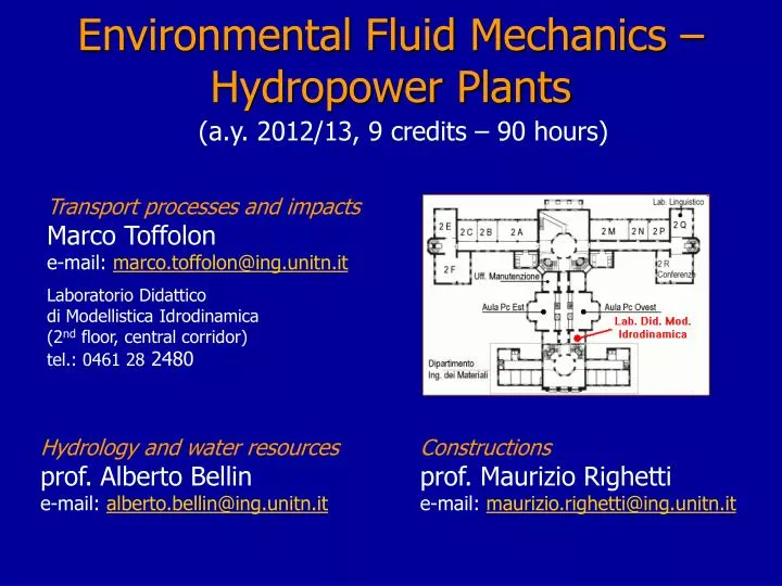
Environmental Fluid Mechanics – Hydropower Plants. ( a.y. 2012/13, 9 credits – 90 hours). Transport processes and impacts Marco Toffolon e-mail: marco.toffolon@ing.unitn.it Laboratorio Didattico di Modellistica Idrodinamica (2 nd floor, central corridor) tel.: 0461 28 2480.

E N D
Environmental Fluid Mechanics – Hydropower Plants (a.y. 2012/13, 9 credits – 90 hours) Transport processes and impacts Marco Toffolon e-mail: marco.toffolon@ing.unitn.it LaboratorioDidattico di ModellisticaIdrodinamica (2nd floor, central corridor) tel.: 0461 28 2480 Hydrology and water resources prof. Alberto Bellin e-mail: alberto.bellin@ing.unitn.it Constructions prof. Maurizio Righetti e-mail: maurizio.righetti@ing.unitn.it
Part II: Transport processes in the environment II-1. Introduction (10 hours) Basic concepts: definition of concentration, mass balance, diffusion. Turbulent mixing. Gaussian model for diffusion processes: basic solution and typical scales. Advection-diffusion equation and analytical solutions in the one-dimensional context. Phases of mixing: near field, intermediate field, far field. Dispersion resulting from non-uniform advection. Dynamics of reactive tracers (including temperature): zero- and one-dimensional models. II-2. Transport processes in rivers and effects of hydropower production (9 hours) Review of basic hydraulic concepts. Estimates of turbulent diffusion and dispersion coefficients. Flood waves due to sudden releases from hydropower plants (hydropeaking). Temperature waves due to the temperature differences between rivers and hydropower releases (thermopeaking). Introduction to river morphology. Hints on biological effects of hydro- and thermo-peaking. Modification of habitats in impacted rivers. Numerical models for longitudinal dispersion: examples. II-3. Thermal dynamics of reservoirs (9 hours) Heat budget in closed basins. Stratification cycle and implications on vertical mixing.Effect of withdrawals and inflows on the temperature profile.Hints on biological aspects and water quality.Numerical models for hydro-thermodynamics of reservoirs: examples.Application to a real case: reservoir management and impact on downstream river. ~28 hours
Main references • Lecture notes. • Suggested textbook (transport processes): • S.A. Socolofsky & G.H. Jirka, dispense del corso Special Topics on Mixing and Transport in the Environment, Texas A&M University, 2005. • Further reading on environmental fluid mechanics: • Fischer H.B., Koh J., List J., Imberger J., Brooks H., Mixing in Inland and Coastal Waters, Academic Press, New York, 1988. • Rutherford J.C., River Mixing, John Wiley & Sons, Chichester, 1994. • J.L. Martin, S.C. McCutcheon, Hydrodynamic and transport for water quality modeling, Lewis Publishers CRC Press • About HP impacts on the environment: • Journal papers link on website: http://www.ing.unitn.it/~toffolon/ (“Materiale didattico”)
Environmental fluid mechanics: An emblematic case Deepwater Horizon oil spill http://earthobservatory.nasa.gov/NaturalHazards/event.php?id=43733 21/04/2010 http://fastfreenews.com/wp-content/uploads/2010/06/gulf-oil-spill1.jpg
Impacts of hydropower production Thermal structure Reservoirs Ecosystems Rivers Sediments Macro-benthos Fishes Infilling Clogging Coasts
Eco-hydraulics in Trento: a multi-disciplinary research group Department of Civil and Environmental Engineering University of Trento, Italy NunzioSiviglia Guido Zolezzi Bruno Maiolini M. Cristina Bruno
Hydropeaking: qualitative description Typical medium-term behaviour: daily cycle + weekly cycle due to the production of peaks of electricity. Stage variations are very rapid (order of cm/min or m/h) both in the rising and in the decreasing phase travelling waves. Simplifying assumption: waves have approximately a square shape. Monday Tuesday Friday Saturday Sunday Sunday Thursday Wednesday
… and what is thermopeaking? temperature of reservoir ≠ temperature of river river Hydropeaking thermal alteration Intensity changes during the year http://www.racine.ra.it/europa/uno/esame2003/terzaf/vcv/html/due.htm
Transport in the environment passive tracer concentration: 3 flow field 2 1 (exceptions: reactive tracer oxygen, nutrients, and temperature) • mass is conserved (non-reactive tracers) • concentration tends to become spatially homogeneous “diffusion”
Diffusion Diffusive flux works against concentration gradient Fick law (1855) Phenomenological explanation: random displacement rightward or leftward N steps (time) 200 “balls”, probability of movement 0.2, single boxes
Main features of diffusive processes 3 2 1 Characteristic dimension of the cloud L(t1) L(t2) L(t3) Self-similar Gaussian solution (1D, infinite domain) with variance ±s 68.3% ±2s 95.5% ±3s 99.7% “mass” between extreme points:
How an advective process becomes diffusive… Molecular diffusion (property of tracer+fluid) Thermal oscillations typical values in water ~ 10-5 cm2/s = 10-9 m2/s in air ~ 10-5 m2/s Turbulence (“random” advection) Turbulent diffusion (property of the flow field, and not of the tracer+fluid) for times long enough (longer than the integral scals of turbulence) Non-uniform advective motion + diffusion orthogonal to the flow Dispersion (combined mechanism) for times long enough (longer than the characteristic scale of orthogonal diffusion)
Dispersion: phenomenological description y u(y) x non-uniform advective motion cloud distortion along x dispersion enhanced “diffusion” along x orthogonal diffusion “compacts” the cloud along y Lagrangian model: following particles deterministic component (assigned flow field) random component (turbulence or thermal oscillation)
Numerical simulation concentration C(x) zoom zoom C(y) particles y y x x particles in the x,y domain
River mixing B hp. shallow water, large width (B>>Y) z Y vertical mixing is much faster than transverse mixing y Mixing phases near field: 3D model, turbulent diffusion (+ molecular) source completed vertical mixing intermediate field: 2D model (depth-averaged), dispersion + turbulent diffusion (+ molecular) completed transverse mixing far field: 1D model (cross-section-averaged), dispersion (+ turbulent diffusion + molecular)
Point source in a river 1/2 flow direction Tracciante rilasciato in un fiume. Il mescolamento verticale viene raggiunto molto velocemente (a distanza di circa 10 volte la profondità); il mescolamento trasversale è molto più lento.
Point source in a river 2/2 Le curve incrementano fortemente il mescolamento trasversale a causa delle correnti secondarie.
Confluence Confluenza di tre fiumi: a sinistra, con una concentrazione molto alta di particolato; al centro con una concentrazione intermedia; a destra (più scuro), più pulito. Contorni ben definiti separano di diversi flussi. [Inn a sinistra, Danubio al centro, Passau DE]
Fasi del problema rio Sorne fiume Adige scarico massa M fase 1: mixing nel rio Sorne fase 2: confluenza fase 3: mixing nell’Adige fase 4: cosa succede a valle?