Download
1 / 27
270 likes | 379 Views
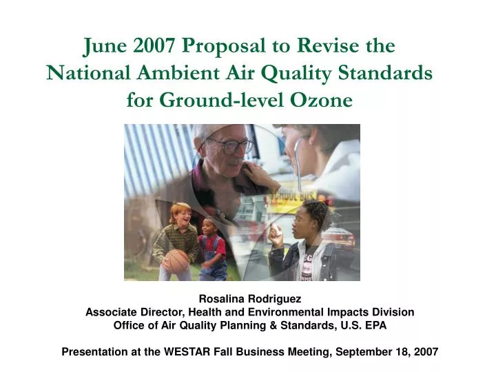
June 2007 Proposal to Revise the National Ambient Air Quality Standards for Ground-level Ozone. Rosalina Rodriguez Associate Director, Health and Environmental Impacts Division Office of Air Quality Planning & Standards, U.S. EPA

E N D
June 2007 Proposal to Revise the National Ambient Air Quality Standards for Ground-level Ozone Rosalina Rodriguez Associate Director, Health and Environmental Impacts Division Office of Air Quality Planning & Standards, U.S. EPA Presentation at the WESTAR Fall Business Meeting, September 18, 2007
Ozone NAAQS Review: Schedule • Proposed rule signed June 20, 2007* • Proposal, RIA, maps, and other supporting materials: http://www.epa.gov/groundlevelozone/ • Public comment period: 90 days, July 11-October 9, 2007 • Public hearings held in Los Angeles and Philadelphia on August 30, and in Atlanta, Chicago, Houston on September 5 • Final rule to be signed by March 12, 2008* (* Dates for proposal and final rules were established under a consent agreement)
Welfare Effects Evidence: Adverse Effects on Vegetation • New studies strengthen conclusions from 1997 review • Plant response to O3 depends on both the cumulative nature of exposures over the growing season and levels of exposure • Studies have focused on exposure metrics that are seasonal and cumulative in nature • Maximum daily 8-hour average concentration metric, upon which the current standard is based, is not an appropriate metric to use to provide protection to sensitive vegetation • Current ambient concentrations in many areas of U.S. are sufficient to cause adverse impacts (e.g., impairment of growth and productivity, foliar injury) on numerous species of trees and crops; problems exist even in areas that attain 1997 8-hour O3 standard of 0.084 ppm • O3 effects on sensitive tree species, including loss of vigor and competitive advantage and susceptibility to disease, could have adverse implications for ecosystems
Welfare Effects Evidence: Adverse Effects on Vegetation • Key sources of information on welfare effects • Concentration response functions from controlled Open-Top Chamber studies on 10 tree species and 14 crop species (100+ studies) • New free air field-based studies on crops (soybeans) and trees (quaking aspen, red maple, birch) support earlier open-top chamber studies • Field-based gradient study in New York City area shows significant biomass loss in cottonwood tree seedlings associated with exposure to ambient O3 concentrations in areas that meet the current standard, including rural areas • National-scale, standardized foliar injury surveys conducted by USDA Forest Service, using formalized monitoring protocols, document widespread injury on sensitive bioindicator plants
Urban Site Rural Site • O3 Gradient Study • (Gregg et al. Nature 2003) • NYC area • Cottonwood trees studied in the field without chambers • Supports open-top chamber results 1.9 ppm-hrs 7.5 ppm-hrs urban rural
Vegetation Risk Assessment • Cumulative O3 exposures were interpolated for the entire U.S. using monitored and CMAQ model information • Interpolation is difficult in the West due to few monitors and complex terrain • The interpolation method performed well when compared to monitors, but generally underestimated W126 exposures in the West • Risks of biomass loss in trees and yield loss in crops were estimated taking into account species specific growing ranges and responses to seasonal O3 exposures • Important known O3 sensitive trees in the West include: quaking aspen, ponderosa pine, black cherry & cottonwood • These trees were shown to have estimated annual biomass losses of up to 19% in some areas of California • Growths losses greater than 2% annually can be significant due to compounding effects over life-time of a tree (Heck & Cowling 1997)
Estimated 12-hr W126 ozone concentration – max 3-months for 2001- “as is” (base case)
Estimated 12-hr W126 ozone concentration – max 3-months for 2001- just meet the 0.084, 8-hr form
Vegetation Risk at Specific Sites in the West • Known O3 sensitive trees such as quaking aspen, cottonwood, and ponderosa pine grow in Canyonlands, UT; Grand Canyon, AZ; and Bandelier, NM • Each of these Class I areas has O3 monitoring and were below the current 8-hr standard in 2003-2005, but had W126 values averaging about 20 ppm-hrs (range 14-24 ppm-hrs) • A W126 of 20 ppm-hrs is estimated to decrease annual growth in quaking aspen and ponderosa pine seedlings by approximately 12% and 8%, respectively • Annual growth losses compound over many seasons and can substantially affect the long-term growth and competitiveness of these species in the ecosystem
CASAC Recommendations: Secondary O3 Standard • “Adverse effects on a wide range of vegetation…are to be expected and have been observed in areas that are below the level of the current 8-hr standard.” • CASAC “encourages the Administrator to establish an alternative cumulative secondary standard… that is distinctly different in averaging time, form and level from the currently existing or potentially revised 8-hr primary standard.” • “…it is not appropriate to try to protect vegetation … by continuing to promulgate identical primary and secondary standards for ozone…” • CASAC recommended a specific cumulative index form called the W126 that would extend over the entire growing season to capture biological impacts • CASAC recommended a standard level of 7-15 ppm-hrs
Proposed Revisions to Secondary Ozone Standard • EPA has proposed two alternatives for revising the secondary standard: • One option would be to establish a new cumulative, seasonal standard expressed as an index of the annual sum of weighted hourly concentrations (using the W126 form) • EPA has proposed to cumulate the index over the 12-hour daylight period (8 am to 8 pm) during the consecutive 3-month period within the ozone season with the maximum index value • EPA has proposed to set the level for this standard within the range of 7 to 21 ppm-hrs • EPA is taking comment on: • Establishing a cumulative, seasonal standard based on a 3-year average, rather than a 1-year average • Establishing a suite of secondary standards based on different ambient levels designed to reflect variation in the significance of ozone-related vegetation effects from a public welfare perspective across type of effect, intended plant use, and location • Another option would be to revise the secondary standard so that it is identical to the proposed primary 8-hour standard (0.070 to 0.075 ppm)
Proposed 12-hr W126 levels • Proposed range: 12-hr, max. 3-mo. W126 of 7 to 21 ppm-hrs • Upper end based on approx. equivalent SUM06 of 25 ppm-hrs (W126 of 21 ppm-hrs) proposed in 1996 expected to provide protection for some agricultural crops and trees • W126 of 21 ppm-hrs expected to provide half of all trees and crops studied (with C-R functions) from a 10% annual biomass or yield loss • However, sensitive trees and crops could have greater losses at that level • Lower end informed by CASAC recommendations and results of a consensus-building workshop (Heck and Cowling, 1997) report that suggest lower ranges* might be more appropriate to consider, especially for natural vegetation: • Crops: 13 to 18 ppm-hrs • Tree seedlings (natural stands): 9-13 ppm-hrs • Foliar injury: 7-11 ppm-hrs (* Ranges in terms of SUM06 originally. Approximate W126 ranges calculated by staff.)
Understanding the W126 Secondary Standard Alternative • Steps in calculating W126 value for a particular site: • Measure hourly ozone (O3) concentrations for each hour within the 12 hour daylight period (8am-8pm). • Assign a weight to each hourly value based on concentration: lower concentrations receive less weight than higher concentrations. • Sum the 12 weighted hourly values to calculate a daily W126 value. • Repeat steps 1-3 for each day within the ozone season and then sum the daily values to calculate the monthly W126 value. • Identify the consecutive 3-month period whose monthly W126 values produce the highest total. • This total becomes the seasonal W126 for this site. weight Example of weighting over 5-hour period: Daily value = Sum of values over 12 daylight hours
CASAC Recommendations: Primary O3 Standard • CASAC unanimously concluded: “no scientific justification for retaining” current standard; standard “needs to be substantially reduced to protect human health, particularly in sensitive subpopulations” • CASAC “unanimously recommends that the current primary O3 NAAQS be revised and that the level that should be considered … be from 0.060 to 0.070 ppm” • Recommended specifying standard level in terms of parts per billion
Proposed Revisions to Primary Ozone Standard • On June 20, EPA proposed to strengthen the health-based standard from 0.084 ppm to a level within the range of 0.070 to 0.075 ppm • The Agency is requesting comment on a range of alternative levels for the standard, down to 0.060 ppm and up to the level of the current standard • EPA also proposes to specify the level of the primary standard to the 3rd decimal (i.e. the nearest thousandth ppm), because of the precision current monitoring technology • Based on the new scientific evidence in this review, the Administrator concluded that the current standard does not adequately protect human health: • Clinical studies show evidence of adverse respiratory responses in healthy adults from exposure to ozone at a level of 0.080 parts per million (ppm); very limited new evidence at 0.060 ppm • Large number of new epidemiological studies, including new multi-city studies, strengthen EPA’s confidence in the links between ozone exposure and health effects. New studies link ozone exposure to important new health effects, including mortality, increased asthma medication use, school absenteeism, and cardiac-related effects • Studies report effects at ozone levels well below the current standard • Studies of people with asthma indicate that they experience larger and more serious responses to ozone that take longer to resolve
Ozone RIA: Overview of Approach • Benefits and costs of attaining 4 alternative primary standards: • 0.079 ppm • 0.075 ppm • 0.070 ppm • 0.065 ppm • Baseline for analysis– 2020 expected air quality after application of: • All final rules (e.g. Clean Air Interstate Rule, the Clean Air Mercury Rule, the Clean Air Visibility Rule, the Clean Air Nonroad Diesel Rule, the Light-Duty Vehicle Tier 2 Rule, the Heavy Duty Diesel Rule, etc) • Projected reductions from forthcoming regulations (e.g. Locomotive and Marine Vessels and for Small Spark-Ignition Engines) • Controls modeled in 2006 PM2.5 RIA for attaining revised PM2.5 standards • Includes limited, targeted EGU controls in the West (CA and Utah) • Controls modeled to bring areas into attainment with 1997 ozone standard (0.08 ppm) • Analytical approach • Modeled hypothetical control scenario to attain a tighter alternative primary standard of 0.070 ppm • For areas not modeled to attain based on application of known controls, extrapolated additional emissions reductions • Based on 0.070 ppm model run, extrapolated results for 0.065, 0.075, 0.079 ppm
Control Measures for O3 Proposal RIA – Western US only [1] Reductions from Ocean-Going Vessels burning diesel fuel were applied in the Base Case analysis. However, we inadvertently omitted the associated reductions that would occur in vessels burning residual fuels. These additional reductions were applied in the Baseline analysis for the east and in the .070 analyses for the east and west. The omission was not identified in time to include it in the initial Baseline analysis for the west, but was included in the Baseline national PM co-benefits analysis for the east and west. [2] Onroad and Nonroad DPF were applied in the baseline, and SCR retrofit technologies were chosen because of the need to reduce NOx emissions..
Current Ozone Nonattainment Area Status (based on 2003-2005 air quality data) • Areas Re-Designated to Maintenance/Attainment Areas (16 Areas*) • Designated Nonattainment Areas Below the Level of the Standard, (58 Areas**) • Designated Nonattainment Areas Above the Level of the Standard, (52 Areas) *1 Area had incomplete data for 2003-2005 **4 Areas had incomplete data for 2003-2005 Attainment Status as of March 19, 2007
Counties With Monitors Violating the Current Primary 8-hour Ozone Standard 0.08 parts per million (Based on 2003 – 2005 Air Quality Data) Notes: 1 104 of 639 monitored counties violate. 2 No monitored counties outside the continental U.S. violate. 3 Monitored data can be obtained from the AQS system at http://www.epa.gov/ttn/airs/airsaqs/ 4 The current standard of 0.08 ppm is effectively expressed as 0.084 ppm when rounding conventions are applied.
Estimates are based on the most recent data (2003 – 2005). EPA will not designate areas as nonattainment on these data, but likely on 2006 - 2008 data which we expect to show improved air quality. Counties With Monitors Violating Alternate 8-hour Ozone Standards 0.070 and 0.075 parts per million 398 counties violate.075 ppm 135 additional counties violate .070 ppm for a total of 533 Notes: 3 Monitored data can be obtained from the AQS system at http://www.epa.gov/ttn/airs/airsaqs/ 1 398 of 639 monitored counties violate 0.075, 533 of 639 monitored counties violate 0.070. 2 No monitored counties outside the continental U.S. violate.
Counties With Monitors Projected to Violate Alternate 8-hour Ozone Standards of 0.070 and 0.075 parts per million in 2020 (Proposal RIA baseline scenario) 82 counties violate 0.075 ppm 121 additional counties violate 0.070 ppm for a total of 203 EPA cannot project future levels for these counties with monitors at this time Notes: 1 Modeled emissions reflect the expected reductions from federal programs including the Clean Air Interstate Rule, the Clean Air Mercury Rule, the Clean Air Visibility Rule, the Clean Air Nonroad Diesel Rule, the Light-Duty Vehicle Tier 2 Rule, the Heavy Duty Diesel Rule, proposed rules for Locomotive and Marine Vessels and for Small Spark-Ignition Engines, and state and local level mobile and stationary source controls identified for additional reductions in emissions for the purpose of attaining the current PM 2.5 and Ozone standards. 2 Controls applied are illustrative. States may choose to apply different control strategies for implementation. 3 Modeled design values in ppm are only interpreted up to 3 decimal places. 4 Consistent with current modeling guidance, EPA did not project 2020 concentrations for counties where 2001 base year concentrations were less than recommended criterion. Such projections may not represent expected future levels. These counties are shown on the map with a grey dot.
Notes: 1 w126 is out of 555 monitored counties in 2005 2 No monitored counties outside the continental U.S. violate 3 Monitored data can be obtained from the AQS system at http://www.epa.gov/ttn/airs/airsaqs/ 4 These estimates are based on the most recent data (2005). EPA will not designate areas as nonattainment on these data, but likely on 2006 - 2008 data which we expect to show improved air quality. Counties With Monitors Violating Alternative w126 Exposure Index Secondary Standards and 8-hour 0.075 Ozone Primary Standard(Based on 2005 Air Quality Data for the w126 and 2003-2005 Air Quality Data for 0.075) 72 counties exceed a standard of 21 using the w126 exposure index 184 additional counties exceed a standard of 15 using the w126 exposure index for a total of 256 220 additional counties exceed a standard of 7 using the w126 exposure index for a total of 476 79 counties meet a standard of 7 using the w126 exposure index for a total of 555 Outlined in heavy black are the 398 counties that exceed the 0.075 alternate 8-hr primary standard
Notes: 1 w126 is out of 555 monitored counties in 2005 2 No monitored counties outside the continental U.S. violate 3 Monitored data can be obtained from the AQS system at http://www.epa.gov/ttn/airs/airsaqs/ 4 These estimates are based on the most recent data (2005). EPA will not designate areas as nonattainment on these data, but likely on 2006 - 2008 data which we expect to show improved air quality. Counties With Monitors Violating Alternative w126 Exposure Index Secondary Standards and 8-hour 0.070 Ozone Primary Standard(Based on 2005 Air Quality Data for the w126 and 2003-2005 Air Quality Data for 0.070) 72 counties exceed a standard of 21 using the w126 exposure index 184 additional counties exceed a standard of 15 using the w126 exposure index for a total of 256 220 additional counties exceed a standard of 7 using the w126 exposure index for a total of 476 79 counties meet a standard of 7 using the w126 exposure index for a total of 555 Outlined in heavy black are the 533 counties that exceed the 0.070 alternate 8-hr primary standard