Download
1 / 16
160 likes | 322 Views
Basic Life Table Computations - I. (Session 12). Learning Objectives. At the end of this and the next session, you will be able to construct a Life Table or abridged Life Table from a given set of mortality data

E N D
Basic Life Table Computations - I (Session 12)
Learning Objectives At the end of this and the next session, you will be able to • construct a Life Table or abridged Life Table from a given set of mortality data • express in words and in symbolic form the connections between the standard columns of the LT • interpret the LT entries and begin to utilise LT thinking in more complex demographic calculations
An Example • Repeated from session 11, below is part of an abridged Life Table (LT) for South African males, published by WHO • The highlighted portion is then pulled out to illustrate some further Life Table calculations. • See your handout for the complete age range.
Computations, not data • Added columns discussed below represent additional calculations built solely on the same original nqx data. • They are further derived values. • Below see graph of nqx vs. x, approximate because rates reflect different age-groups and we have to “scale up” the first two values so their values are comparable with later age groups.
Notes: 1 • Graph shows a local peak in age-group 35-39. This is not historically typical; might arise because in the population from which data are sourced there was a high effect of AIDS in this cohort. • As we go through this session, note how this simple-seeming list of probabilities is manipulated in many ways to generate useful means of expressing information.
Whatis ndx? • ndx is simply the number expected to die in each age range, so can be expressed in several ways e.g. ndx = nqx . lx i.e. the probability of dying in an age-range times the number of people “available to die” at the start of the range ndx = lx - lx+n i.e. the number of people alive and “available to die” at the start of the range minus the number of survivors at the end of the age range
Note that 5d0 was calculated as sum of deaths in ranges 0-1 and 1-4-to put figures on a common scale herein
Why compute ndx?: 1 By looking explicitly at this column we can see how many people are expected to die in each age range which depends on the mortality rate, & on the number left in the LT population. The largest single number in the ndx column (see handout) is 9232 for the age range 35 to 39 inclusive: death rates increase thereafter, but less people are “available to die”
Why compute ndx?: 2 Note that in the age-range 35 to 39, an average of less than 1850 per year are expected to die BUT in the age-range 0-1 year 5077 babies expected to die: nearly 3 times as many on a 1-year basis; AND the babies potentially had their whole life ahead of them: this illustrates the importance of attention to infant health, morbidity and mortality.
Whatis nLx?: 1 nLx is defined as the number of years lived between exact ages x and x+n by members of the Life Table population. Of course the starting number is lx at age x. All those lx+n who survive to age x+n each live n years in the period. A simple assumption is that the (lx- lx+n) who die have each lived n/2 years N.B. not very good assumption e.g. more baby deaths cluster nearer to age 0
Whatis nLx?: 2 On the simple assumption:- nLx = n.lx+n + ½n.[lx- lx+n], which is algebraically equivalent to:- nLx = n[½(lx+ lx+n)]. The expression [½(lx+ lx+n)] can be put into words as the “average population alive in the age range x to x+n”, so another way to express it is:- “over the n-year period, the average population each lived n years”
WhatisL0? We noted that of those who die aged 0, the average age at death is usually much less than 6 months.) A rather better approximation to reality, but still simple, for the first year of life, is:- L0 = .3l0 + 0.7l1 i.e. L0 = l1 + .3(l0 - l1) Note that this counts 0.3 of a year for each child that dies aged 0.
Practical work follows to ensure learning objectives are achieved…